A balanced experimental design is one in which the distribution of the covariates is the same in both the control and treatment groups. However, although often achievable in an experiment, for observational data this ideal is seldom achieved.
The MatchIt package provides a means of pre-processing data so that the treated and control groups are as similar as possible, minimising the dependence between the treatment variable and the other covariates.
I will illustrate this with a simple (and somewhat contrived) example. Consider the following situation: a group of school children is being taught history. A year of 150 children is split between two teachers, Claire and Jane. Jane has some revolutionary ideas about teaching and she claims that she is able to achieve better results than Claire. They set out to test this claim using a set of standardised questions. The results of the questions along with the gender and age of each of the children are recorded. Claire’s husband loads the data into R and it looks like this:
summary(pupils)
 gender      age           teacher       grades
 F:69   Min.   : 9.006   Claire:90   Min.   :28.00
 M:81   1st Qu.: 9.451   Jane  :60   1st Qu.:49.00
        Median : 9.630               Median :59.50
        Mean   : 9.725               Mean   :59.29
        3rd Qu.: 9.942               3rd Qu.:70.00
        Max.   :11.878               Max.   :94.00
with(pupils, table(teacher, gender))
        gender
teacher   F  M
  Claire 32 58
  Jane   37 23
tapply(pupils$age, list(pupils$teacher, pupils$gender), median)
              F        M
Claire 9.539227  9.55096
Jane   9.961180 10.05199
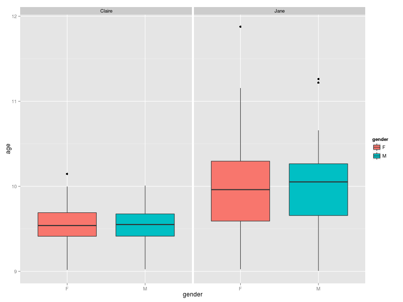
Claire is teaching 90 children, almost two thirds of which are boys. Jane is only teaching 60 children with almost the opposite gender ratio. The distribution of ages is reflected in the plot below. The children taught by Jane have a wider range of ages and their median age is higher than those taught by Claire.
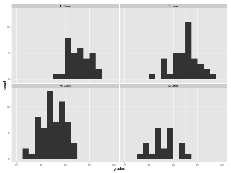
The distribution of the aggregate result of the questions (expressed as a %) are given below. It appears that for both teachers the girls fare better than the boys.
If we make a simple comparison of the average grade for children taught by Claire and Jane, then it seems like Jane might be onto something: her average is about 5% higher than Claire’s.
tapply(pupils$grades, pupils$teacher, mean)
  Claire     Jane
57.17778 62.45000
But that is not the full story: if we break down the averages by gender and teacher then the results are less convincing: boys do slightly better under Jane’s regime, while girls do slightly worse.
tapply(pupils$grades, list(pupils$gender, pupils$teacher), mean)
    Claire     Jane
F 70.81250 69.27027
M 49.65517 51.47826
Let’s apply the tried and tested t-test to see if there is a significant difference between the average grades.
t.test(pupils$grades[pupils$teacher == "Claire"], pupils$grades[pupils$teacher == "Jane"])
	Welch Two Sample t-test

data:  pupils$grades[pupils$teacher == "Claire"] and pupils$grades[pupils$teacher == "Jane"]
t = -2.2626, df = 126.725, p-value = 0.02537
alternative hypothesis: true difference in means is not equal to 0
95 percent confidence interval:
 -9.8833660 -0.6610785
sample estimates:
mean of x mean of y
 57.17778  62.45000
This indicates that the difference in the mean grade for children taught by Claire and Jane is significant at the 5% level (p-value = 0.02537). Perhaps Jane is right? However, contradictory performance of the two genders taken separately should cause us to think carefully about this result. Perhaps the fact that Jane is teaching a larger proportion of girls is having an effect? Or maybe the older children in Jane’s class are skewing the statistics?
This is where MatchIt comes into play. First we add a dichotomous treatment variable, which is 1 for every child taught by Jane and 0 otherwise.
pupils$treatment = ifelse(pupils$teacher == "Jane", 1, 0)
The resulting data is then fed into the matching routine.
(m <- matchit(treatment ~ gender + age, data = pupils, method = "nearest"))
Call:
matchit(formula = treatment ~ gender + age, data = pupils, method = "nearest")

Sample sizes:
          Control Treated
All            90      60
Matched        60      60
Unmatched      30       0
Discarded       0       0
We see that in the original (unmatched) data there were 90 records in the control (Claire) group and only 60 in the treated (Jane) group. After matching there are 60 records in each group. The remaining 30 records are unmatched. We then extract the matched records.
matched <- match.data(m)

with(matched, table(teacher, gender))
        gender
teacher   F  M
  Claire 29 31
  Jane   37 23
tapply(matched$age, list(matched$teacher, matched$gender), median)
              F         M
Claire 9.584322  9.672314
Jane   9.961180 10.051985
The gender and age disparities between the control and treated group have not been removed but they are now much improved. What influence does this have on a comparison of the grades?
t.test(matched$grades[matched$teacher == "Claire"], matched$grades[matched$teacher == "Jane"])
	Welch Two Sample t-test

data:  matched$grades[matched$teacher == "Claire"] and matched$grades[matched$teacher == "Jane"]
t = -0.9127, df = 117.593, p-value = 0.3633
alternative hypothesis: true difference in means is not equal to 0
95 percent confidence interval:
 -7.607438  2.807438
sample estimates:
mean of x mean of y
    60.05     62.45
The difference in average grade is no longer significant. Perhaps Jane has not really discovered anything revolutionary after all? The initial difference in results was probably due to the imbalance between the gender ratios in the control and treatment groups. Certainly the data indicate that there is a marked difference in performance between the girls and boys.
Finally, it seems to me that MatchIt is most effective when the control group is larger than the treatment group. This was the situation for the example above. If the converse applies then MatchIt does not appear to have much of an effect.
Things That Might Go Wrong
Sometimes things might not run quite so smoothly.
- If you get an error message like this then it normally means that the output variable from your model is not dichotomous. You need to make it either a Boolean or 0/1 variable.
Error in weights.matrix(match.matrix, treat, discarded) :
  No units were matched
In addition: Warning messages:
1: glm.fit: algorithm did not converge
2: glm.fit: fitted probabilities numerically 0 or 1 occurred
3: In max(pscore[treat == 0]) :
  no non-missing arguments to max; returning -Inf
4: In max(pscore[treat == 1]) :
  no non-missing arguments to max; returning -Inf
5: In min(pscore[treat == 0]) :
  no non-missing arguments to min; returning Inf
6: In min(pscore[treat == 1]) :
  no non-missing arguments to min; returning Inf