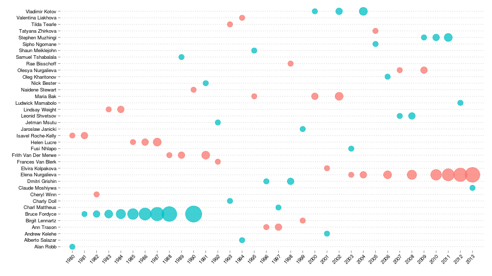
Continuing on my quest to document the Comrades Marathon results, today I have put together a chart showing the winners of both the men and ladies races since 1980. Click on the image below to see a larger version.
The analysis started off with the same data set that I was working with before, from which I extracted only the records for the winners.
winners = subset(results, gender.position == 1, select = c(year, name, gender, race.time))
head(winners)
     year               name gender race.time
1    1980          Alan Robb   Male  05:38:25
428  1980 Isavel Roche-Kelly Female  07:18:00
3981 1981      Bruce Fordyce   Male  05:37:28
4055 1981 Isavel Roche-Kelly Female  06:44:35
7643 1982      Bruce Fordyce   Male  05:34:22
7873 1982        Cheryl Winn Female  07:04:59
I then added in a field which gives a count of the number of times each person won the race.
library(plyr)
winners = ddply(winners, .(name), function(df) {
     df = df[order(df$year),]
     df$count = 1:nrow(df)
     return(df)
})
subset(winners, name == "Bruce Fordyce")
   year          name gender race.time count
7  1981 Bruce Fordyce   Male  05:37:28     1
8  1982 Bruce Fordyce   Male  05:34:22     2
9  1983 Bruce Fordyce   Male  05:30:12     3
10 1984 Bruce Fordyce   Male  05:27:18     4
11 1985 Bruce Fordyce   Male  05:37:01     5
12 1986 Bruce Fordyce   Male  05:24:07     6
13 1987 Bruce Fordyce   Male  05:37:01     7
14 1988 Bruce Fordyce   Male  05:27:42     8
15 1990 Bruce Fordyce   Male  05:40:25     9
The chart was generated as a scatter plot using ggplot2. The size of the points relates to the number of times each person won the race. The colour scale is as you might imagine: pink for the ladies and blue for the men.
library(ggplot2)

ggplot(winners, aes(x = year, y = name, color = gender)) +
  geom_point(aes(size = count), shape = 19, alpha = 0.75) +
  scale_size_continuous(range = c(5, 15)) +
  ylab("") + xlab("") +
  scale_x_discrete(expand = c(0, 1)) +
  theme(
    axis.text.x = element_text(angle = 45, hjust = 1, colour = "black"),
    axis.text.y = element_text(colour = "black"),
    legend.position = "none",
    panel.background = element_blank(),
    panel.grid.major = element_line(linetype = "dotted", colour = "grey"),
    panel.grid.major.x = element_blank()
  )
Two of the key aspects of getting this to look just right were:
- the call to
scale_size_continuous()which ensured that a reasonable range of point sizes was used and - the call to
scale_x_discrete()which expanded the plot very slightly so that the points near the borders were not cropped.