Text Mining the Complete Works of William Shakespeare
I am starting a new project that will require some serious text mining. In the interests of bringing myself up to speed on the {tm} package, I thought I would apply it to the Complete Works of William Shakespeare and just see what falls out.
The first order of business was getting my hands on all that text. Fortunately it is available from a number of sources. I chose to use Project Gutenberg.
TEXTFILE = "data/pg100.txt"
if (!file.exists(TEXTFILE)) {
     dir.create(dirname(TEXTFILE), FALSE)
     download.file("https://www.gutenberg.org/cache/epub/100/pg100.txt", destfile = TEXTFILE)
}
shakespeare = readLines(TEXTFILE)
length(shakespeare)
[1] 124787That’s quite a solid chunk of data: 124787 lines. Let’s take a closer look.
head(shakespeare)[1] "The Project Gutenberg EBook of The Complete Works of William Shakespeare, by"
[2] "William Shakespeare"
[3] ""
[4] "This eBook is for the use of anyone anywhere at no cost and with"
[5] "almost no restrictions whatsoever. You may copy it, give it away or"
[6] "re-use it under the terms of the Project Gutenberg License included"tail(shakespeare)[1] "https://www.gutenberg.org/2/4/6/8/24689" ""
[3] "An alternative method of locating eBooks:" "https://www.gutenberg.org/GUTINDEX.ALL"
[5] "" "*** END: FULL LICENSE ***"There seems to be some header and footer text. We will want to get rid of that! Using a text editor I checked to see how many lines were occupied with metadata and then removed them before concatenating all of the lines into a single long, long, long string.
shakespeare = shakespeare[-(1:173)]
shakespeare = shakespeare[-(124195:length(shakespeare))]

shakespeare = paste(shakespeare, collapse = " ")
nchar(shakespeare)
[1] 5436541While I had the text open in the editor I noticed that sections in the document were separated by the following text:
<<THIS ELECTRONIC VERSION OF THE COMPLETE WORKS OF WILLIAM
SHAKESPEARE IS COPYRIGHT 1990-1993 BY WORLD LIBRARY, INC., AND IS
PROVIDED BY PROJECT GUTENBERG ETEXT OF ILLINOIS BENEDICTINE COLLEGE
WITH PERMISSION.  ELECTRONIC AND MACHINE READABLE COPIES MAY BE
DISTRIBUTED SO LONG AS SUCH COPIES (1) ARE FOR YOUR OR OTHERS
PERSONAL USE ONLY, AND (2) ARE NOT DISTRIBUTED OR USED
COMMERCIALLY.  PROHIBITED COMMERCIAL DISTRIBUTION INCLUDES BY ANY
SERVICE THAT CHARGES FOR DOWNLOAD TIME OR FOR MEMBERSHIP.>>
Obviously that is going to taint the analysis. But it also serves as a convenient marker to divide that long, long, long string into separate documents.
shakespeare = strsplit(shakespeare, "<<[^>]*>>")[[1]]
length(shakespeare)
[1] 218This left me with a list of 218 documents. On further inspection, some of them appeared to be a little on the short side (in my limited experience, the bard is not known for brevity). As it turns out, the short documents were the dramatis personae for his plays. I removed them as well.
(dramatis.personae <- grep("Dramatis Personae", shakespeare, ignore.case = TRUE))[1] 2 8 11 17 23 28 33 43 49 55 62 68 74 81 87 93 99 105 111 117 122 126 134 140 146 152 158
[28] 164 170 176 182 188 194 200 206 212length(shakespeare)[1] 218shakespeare = shakespeare[-dramatis.personae]
length(shakespeare)[1] 182Down to 182 documents, each of which is a complete work.
The next task was to convert these documents into a corpus.
library(tm)

doc.vec <- VectorSource(shakespeare)
doc.corpus <- Corpus(doc.vec)
summary(doc.corpus)
A corpus with 182 text documents
The metadata consists of 2 tag-value pairs and a data frame
Available tags are:
create_date creator
Available variables in the data frame are:
MetaIDMuch of those documents is not relevant to text mining. Before proceeding any further we’ll clean things up a bit. First we convert all of the text to lowercase and then remove punctuation, numbers and common English stopwords. Possibly the list of English stop words is not entirely appropriate for Shakespearean English, but it is a reasonable starting point.
doc.corpus <- tm_map(doc.corpus, content_transformer(tolower))
doc.corpus <- tm_map(doc.corpus, removePunctuation)
doc.corpus <- tm_map(doc.corpus, removeNumbers)
doc.corpus <- tm_map(doc.corpus, removeWords, stopwords("english"))
Next we perform stemming, which removes affixes from words (so, for example, “run”, “runs” and “running” all become “run”).
library(SnowballC)

doc.corpus <- tm_map(doc.corpus, stemDocument)
All of these transformations have resulted in a lot of whitespace, which is then removed.
doc.corpus <- tm_map(doc.corpus, stripWhitespace)If we have a look at what’s left, we find that it’s just the lowercase, stripped down version of the text (which I have truncated here).
inspect(doc.corpus[8])A corpus with 1 text document
The metadata consists of 2 tag-value pairs and a data frame
Available tags are:
create_date creator
Available variables in the data frame are:
MetaID
[[1]]
act ii scene messina pompey hous enter pompey menecr mena warlik manner pompey great god just shall
assist deed justest men menecr know worthi pompey delay deni pompey while suitor throne decay thing
sue menecr ignor beg often harm wise powr deni us good find profit lose prayer pompey shall well
peopl love sea mine power crescent augur hope say will come th full mark antoni egypt sit dinner
will make war without door caesar get money lose heart lepidus flatter flatterd neither love eitherThis is where things start to get interesting. Next we create a Term Document Matrix (TDM) which reflects the number of times each word in the corpus is found in each of the documents.
(TDM <- TermDocumentMatrix(doc.corpus))A term-document matrix (18651 terms, 182 documents)
Non-/sparse entries: 182898/3211584
Sparsity : 95%
Maximal term length: 31
Weighting : term frequency (tf)inspect(TDM[1:10,1:10])A term-document matrix (10 terms, 10 documents)
Non-/sparse entries: 1/99
Sparsity : 99%
Maximal term length: 9
Weighting : term frequency (tf)
Docs
Terms 1 2 3 4 5 6 7 8 9 10
aaron 0 0 0 0 0 0 0 0 0 0
abaissiez 0 0 0 0 0 0 0 0 0 0
abandon 0 0 0 0 0 0 0 0 0 0
abandond 0 1 0 0 0 0 0 0 0 0
abas 0 0 0 0 0 0 0 0 0 0
abashd 0 0 0 0 0 0 0 0 0 0
abat 0 0 0 0 0 0 0 0 0 0
abatfowl 0 0 0 0 0 0 0 0 0 0
abbess 0 0 0 0 0 0 0 0 0 0
abbey 0 0 0 0 0 0 0 0 0 0The extract from the TDM shows, for example, that the word “abandond” occurred once in document number 2 but was not present in any of the other first ten documents. We could have generated the transpose of the DTM as well.
DTM <- DocumentTermMatrix(doc.corpus)
inspect(DTM[1:10,1:10])
A document-term matrix (10 documents, 10 terms)
Non-/sparse entries: 1/99
Sparsity : 99%
Maximal term length: 9
Weighting : term frequency (tf)
Terms
Docs aaron abaissiez abandon abandond abas abashd abat abatfowl abbess abbey
1 0 0 0 0 0 0 0 0 0 0
2 0 0 0 1 0 0 0 0 0 0
3 0 0 0 0 0 0 0 0 0 0
4 0 0 0 0 0 0 0 0 0 0
5 0 0 0 0 0 0 0 0 0 0
6 0 0 0 0 0 0 0 0 0 0
7 0 0 0 0 0 0 0 0 0 0
8 0 0 0 0 0 0 0 0 0 0
9 0 0 0 0 0 0 0 0 0 0
10 0 0 0 0 0 0 0 0 0 0Which of these proves to be most convenient will depend on the relative number of documents and terms in your data.
Now we can start asking questions like: what are the most frequently occurring terms?
findFreqTerms(TDM, 2000)[1] "come" "enter" "good" "king" "let" "lord" "love" "make" "man" "now" "shall" "sir" "thee"
[14] "thi" "thou" "well" "will"Each of these words occurred more that 2000 times.
What about associations between words? Let’s have a look at what other words had a high association with “love”.
findAssocs(TDM, "love", 0.8)beauti eye
0.83 0.80Well that’s not too surprising!
From our first look at the TDM we know that there are many terms which do not occur very often. It might make sense to simply remove these sparse terms from the analysis.
TDM.common = removeSparseTerms(TDM, 0.1)
dim(TDM)
[1] 18651 182dim(TDM.common)[1] 71 182From the 18651 terms that we started with, we are now left with a TDM which considers on 71 commonly occurring terms.
inspect(TDM.common[1:10,1:10])A term-document matrix (10 terms, 10 documents)
Non-/sparse entries: 94/6
Sparsity : 6%
Maximal term length: 6
Weighting : term frequency (tf)
Docs
Terms 1 2 3 4 5 6 7 8 9 10
act 1 4 7 9 6 3 2 14 1 0
art 53 0 9 3 5 3 2 17 0 6
away 18 5 8 4 2 10 5 13 1 7
call 17 1 4 2 2 1 6 17 3 7
can 44 8 12 5 10 6 10 24 1 5
come 19 9 16 17 12 15 14 89 9 15
day 43 2 2 4 1 5 3 17 2 3
enter 0 7 12 11 10 10 14 87 4 6
exeunt 0 3 8 8 5 4 7 49 1 4
exit 0 6 8 5 6 5 3 31 3 2Finally we are going to put together a visualisation. The TDM is stored as a sparse matrix. This was an apt representation for the initial TDM, but the reduced TDM containing only frequently occurring words is probably better stored as a normal matrix. We’ll make the conversion and see.
library(slam)

TDM.dense <- as.matrix(TDM.common)

TDM.dense
object.size(TDM.common)
207872 bytesobject.size(TDM.dense)112888 bytesAs it turns out the sparse representation was actually wasting space! (This will generally not be true though: it will only apply for a matrix consisting of just the common terms).
These data can be visualised in various ways, but we’ll only look at only two of them. Let’s start with a simple word cloud.
library(wordcloud)

library(RColorBrewer)
palette <- brewer.pal(9,"BuGn")[-(1:4)]

wordcloud(rownames(TDM.dense), rowSums(TDM.dense), min.freq = 1, color = palette)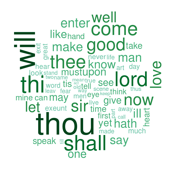
To produce the other plot we first need to convert the data into a tidier format.
library(reshape2)

TDM.dense = melt(TDM.dense, value.name = "count")
head(TDM.dense)
Terms Docs count
1 act 1 1
2 art 1 53
3 away 1 18
4 call 1 17
5 can 1 44
6 come 1 19It’s then an easy matter to use ggplot2 to make up an attractive heat map.
library(ggplot2)

ggplot(TDM.dense, aes(x = Docs, y = Terms, fill = log10(count))) +
     geom_tile(colour = "white") +
     scale_fill_gradient(high="#FF0000" , low="#FFFFFF")+
     ylab("") +
     theme(panel.background = element_blank()) +
     theme(axis.text.x = element_blank(), axis.ticks.x = element_blank())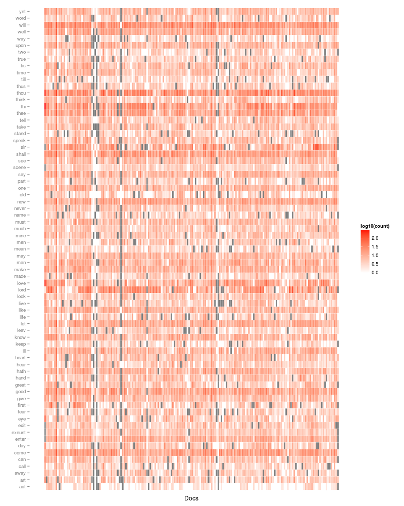
The colour scale indicates the number of times that each of the terms cropped up in each of the documents. I applied a logarithmic transform to the counts since there was a very large disparity in the numbers across terms and documents. The grey tiles correspond to terms which are not found in the corresponding document.
One can see that some terms, like “will” turn up frequently in most documents, while “love” is common in some and rare or absent in others.
That was interesting. Not sure that I would like to make any conclusions on the basis of the results above (Shakespeare is well outside my field of expertise!), but I now have a pretty good handle on how the tm package works. As always, feedback will be appreciated!
References
- Build a search engine in 20 minutes or less.
- Feinerer, I. (2013). Introduction to the tm Package: Text Mining in R.
- Feinerer, I., Hornik, K., & Meyer, D. (2008). Text Mining Infrastructure in R. Journal of Statistical Software, 25(5).