Does the transition to and from Daylight Saving Time (DST) have a (significant) effect on the stock market?
In a recent blog post on The UK Stock Market Almanac, the author found that the average return of the FTSE100 index for the days following the start of British Summer Time (BST) was -0.07% during the interval 1985-2013. This was lower than both the average for all days during this interval (+0.03%) and for all Mondays during this interval (-0.01%). Is this difference significant?
Some History
An article by M. J. Kamstra, L. A. Kramer, and M. D. Levi [1] concluded that:
- the transitions to and from DST have significant effects on the market, a factor of 2 to 5 times larger than the normal weekend effect;
- the change in autumn (reverting to “normal” time) has a greater effect than the change in spring (transition to “summer time”).
It’s probably not possible to base a winning strategy on this effect, but it’s worth taking a closer look at the data.
Grabbing Data on Daylight Saving Time
The first thing that we need is the set of dates for the DST transitions. These are available from the National Physical Laboratory web site and I am going to use the XML library to scape the data.
library(XML)

URL = "https://www.npl.co.uk/educate-explore/what-is-time/archive-of-summer-time-dates-1916-2006"
#
bst.dates = readHTMLTable("data/summer-time-dates.html", which = 1, trim = TRUE, stringsAsFactors = FALSE)[-1,]
#
names(bst.dates) <- c("year", "began", "ended")
#
bst.dates <- transform(
  bst.dates,
  began = paste(began, year),
  ended = paste(ended, year)
)
#
bst.dates$year <- NULL
#
head(bst.dates)
2   21 May 1916    1 October 1916
3  8 April 1917 17 September 1917
4 24 March 1918 30 September 1918
5 30 March 1919 29 September 1919
6 28 March 1920   25 October 1920
7  3 April 1921    3 October 1921
These dates are the Sundays on which the transitions took place. We are interested in the effect on the following day, so we advance them by one day.
for (n in 1:2) {
 bst.dates[,n] = as.Date(bst.dates[,n], format = "%d %B %Y") + 1
}
#
bst.dates = bst.dates[complete.cases(bst.dates),]
#
head(bst.dates)
       began      ended
2 1916-05-22 1916-10-02
3 1917-04-09 1917-09-18
4 1918-03-25 1918-10-01
5 1919-03-31 1919-09-30
6 1920-03-29 1920-10-26
7 1921-04-04 1921-10-04
Grabbing Data on Market Indices
We will take a look at the effect in the British and American stock market, using the FTSE100 and S&P500 indices as indicators.
library(Quandl)

Quandl.auth("xxxxxxxxxxxxxxxxxxxx")

fractional.returns <- function(x) {
  c(NA, diff(x) / x[-length(x)])
}

retrieve.index <- function(code) {
  data = Quandl(
    code,
    start_date = min(bst.dates$began) - 1,
    end_date = max(bst.dates$ended) + 1
  )
  #
  # Re-order so that dates increases
  #
  data = data[order(data$Date),]

  data$returns = fractional.returns(data$Close)
  #
  data = data[, c("Date", "returns")]
  #
  data = data[complete.cases(data),]

  rownames(data) = 1:nrow(data)

  data
}

SP500 <- retrieve.index("YAHOO/INDEX_GSPC")
FTSE100 <- retrieve.index("YAHOO/INDEX_FTSE")

head(FTSE100)
1 1984-04-03 -0.01146106
2 1984-04-04  0.00000000
3 1984-04-05  0.00620778
4 1984-04-06 -0.00535293
5 1984-04-09  0.00036486
6 1984-04-10  0.00793289
We now have two data structures, one for each index. To make the analysis easier, we will consolidate these into a single structure.
indices <- merge(SP500, FTSE100, by.x = "Date", by.y = "Date", all = TRUE)
#
names(indices) <- c("date", "SP500", "FTSE100")
#
indices$year = as.integer(strftime(indices$date, format = "%Y"))
#
indices <- indices[, c(4, 1, 2, 3)]

head(indices)
  year       date      SP500 FTSE100
1 1950 1950-01-04  0.0114046      NA
2 1950 1950-01-05  0.0047478      NA
3 1950 1950-01-06  0.0029533      NA
4 1950 1950-01-09  0.0058893      NA
5 1950 1950-01-10 -0.0029274      NA
6 1950 1950-01-11  0.0035232      NA
The missing values for FTSE100 are because our data for this index only begin in 1984. The data are not currently in a “tidy” format, but that is easily remedied.
library(reshape2)

indices = melt(indices, id.vars = c("year", "date"), variable.name = "index",
               value.name = "returns")

head(indices)
  year       date index    returns
1 1950 1950-01-04 SP500  0.0114046
2 1950 1950-01-05 SP500  0.0047478
3 1950 1950-01-06 SP500  0.0029533
4 1950 1950-01-09 SP500  0.0058893
5 1950 1950-01-10 SP500 -0.0029274
6 1950 1950-01-11 SP500  0.0035232
Plotting Indices
Let’s take a global look at the distribution of the returns.
ggplot(indices) +
  geom_histogram(aes(x = returns), binwidth = 0.005) +
  xlab("Returns") + ylab("") +
  scale_x_continuous(labels = percent_format()) +
  facet_wrap(~ index, ncol = 1) +
  theme_classic()
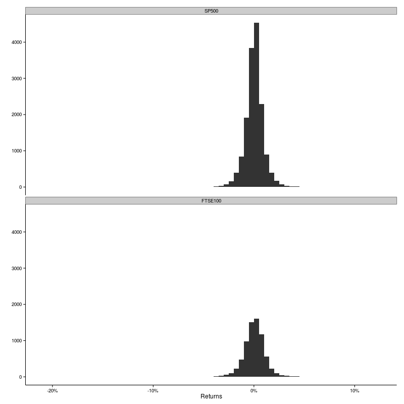
That’s not terribly illuminating. The distributions both look more or less symmetric around 0%. There are fewer counts for the FTSE100 because the data does not go as far back as the S&P500. The scale on the x-axis hints that there are some large outliers, but they are rare and don’t even show up on the histograms.
ggplot(indices, aes(x = year, y = returns, group = year)) +
  geom_boxplot() +
  xlab("") + ylab("Returns") +
  scale_x_continuous(breaks = seq(1940, 2020, 10)) +
  scale_y_continuous(labels = percent_format()) +
  facet_wrap(~ index, ncol = 1) +
  theme_classic()
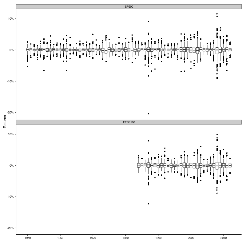
Now that’s a lot more interesting. We can see that the level of variability changes appreciably from year to year. 1987 and 2008 are particularly volatile years. And the massive negative return in 1987 is the Black Monday event of 19 October 1987.
Okay, let’s focus our attention on the returns for the DST transitions. First we’ll merge the index and DST date data. I am sure that there is a more elegant way of doing it, but this gets the job done.
bst.dates.began = merge(bst.dates, indices, by.x = "began", by.y = "date")
bst.dates.began$type = "began"
names(bst.dates.began)[1] = "date"
bst.dates.began[,2] <- NULL
bst.dates.ended = merge(bst.dates, indices, by.x = "ended", by.y = "date")
bst.dates.ended$type = "ended"
names(bst.dates.ended)[1] = "date"
bst.dates.ended[,2] <- NULL
#
bst.dates = rbind(bst.dates.began, bst.dates.ended)[, c(2, 1, 5, 3, 4)]

head(bst.dates)
  year       date  type   index    returns
1 1950 1950-04-17 began   SP500 -0.0044543
2 1950 1950-04-17 began FTSE100         NA
3 1951 1951-04-16 began FTSE100         NA
4 1951 1951-04-16 began   SP500 -0.0022635
5 1952 1952-04-21 began   SP500  0.0080851
6 1952 1952-04-21 began FTSE100         NA
We are going to make comparisons of the returns on the DST transition days to the average returns for the corresponding year. So we gather the summary parameters for each of the indices, grouped by year.
library(plyr)

indices.annual = ddply(indices, .(year, index), summarize,
                        ret.mean = mean(returns, na.rm = TRUE),
                        ret.sd = sd(returns, na.rm = TRUE))

head(indices.annual)
  year   index   ret.mean    ret.sd
1 1950   SP500 0.00086731 0.0094050
2 1950 FTSE100        NaN        NA
3 1951   SP500 0.00063127 0.0067907
4 1951 FTSE100        NaN        NA
5 1952   SP500 0.00045787 0.0049775
6 1952 FTSE100        NaN        NA
Next we merge these back into the DST data and form a new standardised variable for the returns.
bst.dates = merge(bst.dates, indices.annual)

bst.dates = transform(
  bst.dates,
  z = (returns - ret.mean) / ret.sd,
  type = factor(type, labels = paste("DST", c("began", "ended")))
)
head(bst.dates)
  year   index       date      type    returns   ret.mean   ret.sd         z
1 1950 FTSE100 1950-04-17 DST began         NA        NaN       NA        NA
2 1950 FTSE100 1950-10-23 DST ended         NA        NaN       NA        NA
3 1950   SP500 1950-04-17 DST began -0.0044543 0.00086731 0.009405 -0.565833
4 1950   SP500 1950-10-23 DST ended  0.0000000 0.00086731 0.009405 -0.092218
5 1951 FTSE100 1951-04-16 DST began         NA        NaN       NA        NA
6 1951 FTSE100 1951-10-22 DST ended         NA        NaN       NA        NA
Finally we are ready to make a plot.
ggplot(bst.dates, aes(x = z)) +
  geom_histogram(aes(y = ..density..), binwidth = 0.25, fill = "grey") +
  geom_density(adjust = 1.5) +
  geom_vline(aes(xintercept = median), ddply(bst.dates, .(index, type), summarize,
                                        median = median(z, na.rm = TRUE))) +
  geom_vline(xintercept = 0, bst.dates.summary, linetype = "dashed") +
  xlab("") + ylab("") +
  scale_x_continuous(limits = c(-6, 3)) +
  facet_grid(type ~ index) +
  theme_classic()
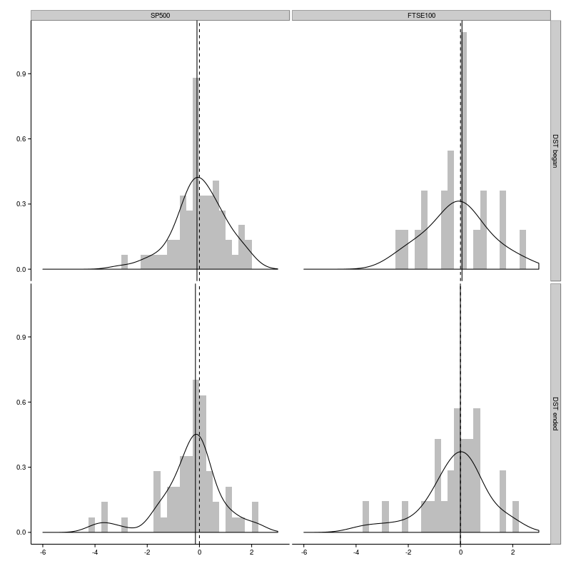
For each index there are two panels, the top one indicates the distribution of standardised returns for the beginning of DST and the lower one for the end of DST. It’s interesting to note that there is a sharp peak at zero for both indices at the beginning of DST. This peak is absent at the end of DST.
The density curves all indicate that the distributions are negatively skewed. The skewness is mostly due to a few large negative outliers. We can find out when these outliers occurred.
ddply(bst.dates, .(index, type), function(df) {head(df[order(df$z),])})
   year   index       date      type    returns    ret.mean    ret.sd        z
1  1980   SP500 1980-03-17 DST began -0.0300673  0.00096039 0.0103718 -2.99156
2  2009   SP500 2009-03-30 DST began -0.0348187  0.00098347 0.0171879 -2.08298
3  1997   SP500 1997-03-31 DST began -0.0216571  0.00113332 0.0114215 -1.99539
4  2003   SP500 2003-03-31 DST began -0.0177417  0.00098699 0.0107516 -1.74195
5  1991   SP500 1991-04-01 DST began -0.0104472  0.00096384 0.0090074 -1.26686
6  1987   SP500 1987-03-30 DST began -0.0234019  0.00029677 0.0202469 -1.17048
7  1997   SP500 1997-10-27 DST ended -0.0686568  0.00113332 0.0114215 -6.11040
8  1987   SP500 1987-10-26 DST ended -0.0827895  0.00029677 0.0202469 -4.10365
9  1951   SP500 1951-10-22 DST ended -0.0244425  0.00063127 0.0067907 -3.69239
10 1982   SP500 1982-10-25 DST ended -0.0396888  0.00060988 0.0115004 -3.50412
11 1955   SP500 1955-10-03 DST ended -0.0270208  0.00097713 0.0096678 -2.89600
12 2001   SP500 2001-10-29 DST ended -0.0238184 -0.00047153 0.0135793 -1.71929
13 2009 FTSE100 2009-03-30 DST began -0.0348816  0.00089709 0.0147533 -2.42514
14 2003 FTSE100 2003-03-31 DST began -0.0256708  0.00057910 0.0122425 -2.14416
15 1988 FTSE100 1988-03-28 DST began -0.0121048  0.00021246 0.0079013 -1.55888
16 2006 FTSE100 2006-03-27 DST began -0.0106191  0.00043522 0.0079146 -1.39669
17 1987 FTSE100 1987-03-30 DST began -0.0225509  0.00022005 0.0166662 -1.36630
18 2007 FTSE100 2007-03-26 DST began -0.0074928  0.00020745 0.0109820 -0.70117
19 1987 FTSE100 1987-10-26 DST ended -0.0618873  0.00022005 0.0166662 -3.72655
20 1997 FTSE100 1997-10-27 DST ended -0.0260553  0.00091785 0.0095248 -2.83187
21 2011 FTSE100 2011-10-31 DST ended -0.0277086 -0.00013775 0.0134164 -2.05501
22 2001 FTSE100 2001-10-29 DST ended -0.0197934 -0.00061135 0.0132487 -1.44785
23 1995 FTSE100 1995-10-23 DST ended -0.0056034  0.00075429 0.0061787 -1.02897
24 1993 FTSE100 1993-10-25 DST ended -0.0044389  0.00074358 0.0062907 -0.82383
So, for both indices the large outliers at the end of DST occurred on 1987-10-26 and 1997-10-27. These dates agree with the outlier dates identified by Pinegar [2].
The skewed distributions only result in an appreciable shift in the median (indicated by the solid vertical line in the plots) for the S&P500 index at the end of DST. In the other three cases the median is very close to zero. Do the standardised returns differ significantly from zero? We can have a look at the Wilcoxon and t-tests.
ddply(bst.dates, .(index, type), summarize,
       t.test = t.test(z, na.rm = TRUE)$p.value,
       wilcox.test = wilcox.test(z, na.rm = TRUE)$p.value)
    index      type   t.test wilcox.test
1   SP500 DST began 0.883197    0.765592
2   SP500 DST ended 0.017311    0.019783
3 FTSE100 DST began 0.637718    0.823729
4 FTSE100 DST ended 0.723530    0.717209
The resulting p-values agree with the qualitative analysis: there is only a significant difference (at the 5% level) for S&P500 at the end of DST (agreeing with [1]).
Spring 2014 DST Transition
As it happens, we have just had a Spring DST transition. Below are the data for the S&P500 and FTSE100 indices for the last two trading days, retrieved from Yahoo! Finance.
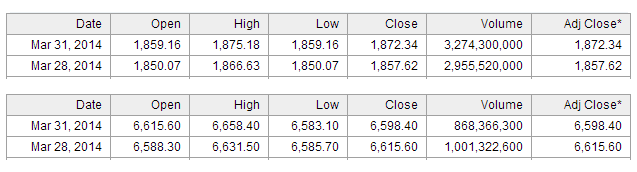
Let’s have a look at the returns.
fractional.returns(c(1857.62, 1872.34))
[1] NA 0.007924118
fractional.returns(c(6615.60, 6598.40))
[1] NA -0.002599915
That’s interesting: the S&P500 index experienced a positive return, while the return on the FTSE100 was negative. We know from the analysis above that the return associated with the DST transition can go either way. We also know that the significant effect on the S&P500 is observed for the Autumn rather than Spring transition, so the results from the weekend are not surprising.
References
- M. J. Kamstra, L. A. Kramer, and M. D. Levi, “Losing Sleep at the Market: The Daylight Saving Anomaly,” Am. Econ. Rev., vol. 90, no. 4, pp. 1005–1011, 2000.
- J. M. Pinegar, “Losing Sleep at the Market: Comment,” Am. Econ. Rev., vol. 92, no. 4, pp. 1251–1256, 2002.
- M. J. Kamstra, L. A. Kramer, and M. D. Levi, “Losing Sleep at the Market: The Daylight Saving Anomaly: Reply,” Am. Econ. Rev., vol. 92, no. 4, pp. 1257–1263, 2002.