Myfxbook provides an interface to your FOREX trading accounts as well as an active trading community.
It has a broad range of functionality including
- a responsive interface to the FOREX market;
- tools for performing statistical analyses on your trades;
- the facility to mirror trades from other traders or systems; and
- provides a platform for publicising trading systems.
R Interface to the API
The API facilitates direct programmatic access to your Myfxbook account. You access the API via HTTP GET requests and it returns the results either as XML or JSON. I have taken advantage of R’s web technologies to build an interface with Myfxbook. I implemented the interface as a reference class which exercises most of the calls in the API.
The first thing we need to do is connect to Myfxbook. To do this we create an instance of the reference class. The class constructor takes an email address and password as arguments. The API returns a session identifier which is then retained as a data member in the class. For security reasons the email address and password are not retained.
fx <- myfxbook$new(email = "xxxxxx@xxxxxxx.xxx", password = "xxxxx", debug = FALSE)
fx
Reference class object of class "myfxbook"
Field "debug":
[1] FALSE
Field "session":
[1] "Xuq0yAJBOrCu9PfI2EWC186040"
We can get the details for the accounts which we have linked to the system. I have just hooked up a single demo account for the purposes of this article.
fx$my.accounts()
      id         name description accountId gain absGain daily monthly
2 893887 Demo Account                625546    0       0     0       0
  withdrawals deposits interest profit balance drawdown equity equityPercent
2           0     5000        0      0    5000     0.48 4985.8         99.72
  demo   lastUpdateDate     creationDate   firstTradeDate tracking views
2 TRUE 04/15/2014 05:55 04/15/2014 02:45 04/14/2014 00:00        0     0
  commission currency profitFactor pips invitationUrl    server
2          0      USD            0    0               Alpari UK
And we can also see the status of other accounts which we are watching.
fx$watched.accounts()
               name    gain drawdown  demo  change
2  Asset management 2004.80    20.24 FALSE 2004.80
21        berezhnoi 3708.64    42.01 FALSE 3708.64
3  Forex Growth Bot  272.39    93.13 FALSE  243.41
4        WallStreet  455.67    27.95 FALSE  455.67
An interface to the community outlook data gives an indication of the number and volume of trades as a function of currency pair.
outlook = fx$outlook()
dim(outlook)
[1] 57 10
head(outlook)
      name shortPercentage longPercentage shortVolume longVolume longPositions shortPositions totalPositions avgShortPrice avgLongPrice
2   EURUSD              65             34     7619.43    4041.45         12449          21054          11660        1.3687       1.3844
210 GBPUSD              61             38     3235.93    1999.51          6612          11440           5235        1.6478       1.6714
3   USDJPY              45             54     1444.90    1732.04          4831           3977           3176      101.0527     102.7562
4   GBPJPY              55             44      642.58     520.81          1376           1798           1163      167.0348     171.1947
5   USDCAD              50             49     1176.98    1138.17          3631           4135           2315        1.0875       1.1046
6   EURAUD              41             58      220.25     314.09           988            822            534        1.4332       1.4994
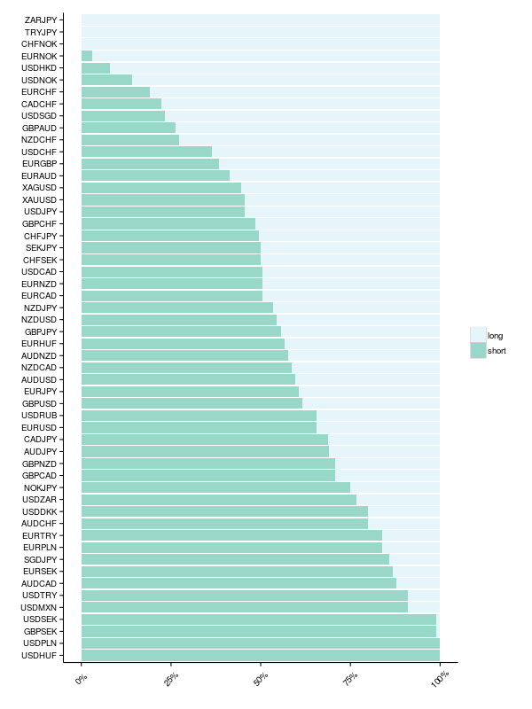
To get a feeling for the relative proportion of long and short trades across all currencies we can put together an informative plot. It requires a little leg work first though to get the data into a workable format:
- melt the data frame into a “tidy” format, extracting only the columns for the percentage of long and short trades;
- normalise the percentages (given as integers which do not all sum to 100%);
- remove entries with missing data;
- neaten up labels for long and short percentages; and
- sort according to fraction of shorts.
outlook.percents = melt(outlook, id.vars = "name",
                        measure.vars = paste0(c("short", "long"), "Percentage"))
outlook.percents = ddply(outlook.percents, .(name), function(df) {
  df$value = df$value / sum(df$value)
  df
})
outlook.percents = outlook.percents[complete.cases(outlook.percents),]
outlook.percents = transform(
  outlook.percents,
  variable = sub("Percentage", "", variable),
  name = reorder(name, outlook.percents$value, function(x) {x[2]})
)
ggplot(outlook.percents, aes(x = name, y = value)) +
   geom_bar(aes(fill = variable), stat = "identity") +
   xlab("") + ylab("") +
   coord_flip() +
   scale_y_continuous(labels = percent_format()) +
   scale_fill_brewer(name = "", palette="BuGn") +
   theme_classic() +
   theme(axis.text.x = element_text(angle = 45, vjust = 0.5))
The outlook data can also be broken down by country for a single currency pair.
outlook = fx$outlook.country("EURUSD")
dim(outlook)
[1] 159 6
head(outlook)
            name code longVolume shortVolume longPositions shortPositions
2        GERMANY   DE      39.23      138.65           495            818
210 BAHAMAS, THE   BS       0.00        0.00             0              0
3         GREECE   GR       0.70        4.19             5             76
4       ANGUILLA   AI       0.00        0.00             0              0
5         BHUTAN   BT       0.00        0.00             0              0
6          JAPAN   JP      19.10       28.03            86            132
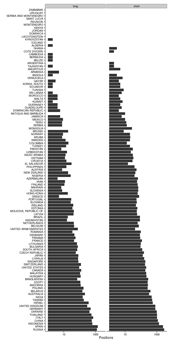
As before, making sense of this is aided by a visualisation. Below is a plot showing the number of long and short positions on EURUSD for a range of countries. We can see that overall the most trades have originated in Spain and Russia and that the majority of these positions are shorts.
We can also get a list of our open trades and pending orders.
fx$open.trades(893887)
          openTime symbol action openPrice     tp      sl profit pips  swap magic
1 04/15/2014 05:46 EURUSD    Buy   1.38166 1.3867 1.37866  54.25 21.7 -0.13     0
2 04/16/2014 08:06 AUDUSD    Buy   0.93722 0.0000 0.92594  -0.75 -0.3  3.60     0
  size.type size.value
1      lots       0.25
2      lots       0.25
fx$open.orders(893887)
          openTime symbol    action openPrice tp sl size.type size.value
1 04/15/2014 05:47 USDJPY Buy Limit     101.3  0  0      lots       0.25
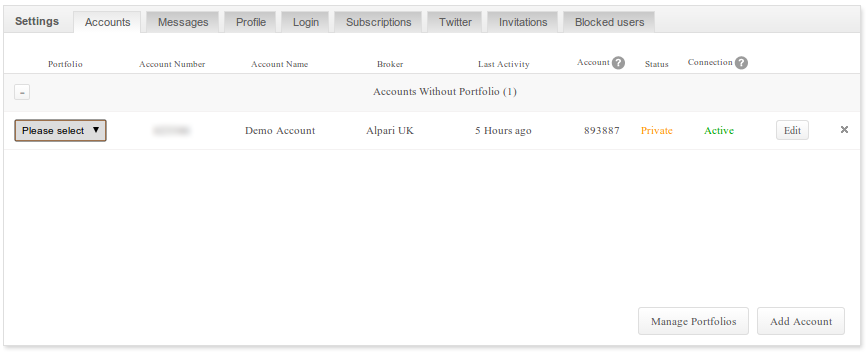
Here the argument is a Myfxbook account number, which is either found on your dashboard (see image below) or from the id field in the output from my.accounts() above.
Daily changes in the account balance can also be retrieved.
fx$daily.gain(893887, "2014-04-01", "2014-04-17")
         date value profit
2  04/14/2014   0.0   0.00
21 04/15/2014  -1.1 -55.16
22 04/16/2014   2.9 200.00
And full details of all transactions can be obtained as a history.
fx$history(893887)
          openTime        closeTime symbol  action openPrice closePrice      tp      sl pips  profit interest commission size.type size.value comment
1 04/16/2014 08:04 04/16/2014 11:30 GBPUSD     Buy   1.67254    1.68054 1.68054 1.66554   80  200.00        0          0      lots       0.25    <NA>
2 04/15/2014 08:03 04/15/2014 15:25 AUDUSD     Buy   0.93931    0.93731 0.94181 0.93731  -20  -50.00        0          0      lots       0.25    <NA>
3 04/15/2014 13:28 04/15/2014 13:28 USDJPY     Buy 101.84000  101.82000 0.00000 0.00000   -2   -5.16        0          0      lots       0.25    <NA>
4 04/14/2014 13:40 04/14/2014 13:40        Deposit   0.00000    0.00000      NA      NA    0 5000.00        0          0      lots            Deposit
Conclusion
I am quite happy with this functionality and I will be using it in one of my current projects. If there is sufficient interest, I will package it up and stick it on CRAN.