With this year’s Comrades Marathon just less than a month away, I was reminded of a story from earlier in the year. Mark Dowdeswell, a statistician at Wits University, found evidence of cheating by some middle and back of the pack Comrades runners. He identified a group of 20 athletes who had suspicious negative splits: they ran much faster in the second half of the race. There was one runner in particular whose splits were just too good to be true. When the story was publicised, this particular runner claimed that it was a conspiracy.
This story emerged in February this year.
There was quite a fuss.
And then everything went quiet. The suspected runners were instructed to attend disciplinary hearings, but the outcomes of these hearings have not been publicised nor have the names of the suspected runners been released.
I have done some previous analyses using Comrades Marathon data. Here I am going to use the same data set to explore these suspicious negative splits.
Data Preparation
I started off by extracting a subset of the columns from my splits data.
split.ratio = splits[, c("year", "race.number", "key", "drummond.time", "race.time")]
tail(split.ratio)
          year race.number      key drummond.time race.time
2013-9911 2013        9911 eb4b3b0c        303.40    686.68
2013-9912 2013        9912 c8d6cfdd        218.73    484.00
2013-9940 2013        9940 f46204ad        249.87    582.03
2013-9954 2013        9954 4bd1ca76        307.62    669.23
2013-9955 2013        9955 b2b9ed60        286.85    651.87
2013-9964 2013        9964 6f14470d        242.20    573.78
The resulting records have fields for the year, athlete’s race number, a unique key identifying the runner, and time taken (in minutes) to reach the little town of Drummond (the half way point at around the marathon distance) and the finish. We will only keep the complete records (valid entries for both half way and the full distance) and then add a new field.
# This is derived from (race.time - drummond.time) / drummond.time - 1
#
split.ratio = transform(
  split.ratio,
  ratio = race.time / drummond.time - 2
)
head(split.ratio)
           year race.number      key drummond.time race.time   ratio
2000-10003 2000       10003 f1dffb06        243.65    532.33 0.18483
2000-10009 2000       10009 b06cab7f        274.47    599.95 0.18588
2000-10010 2000       10010 929fd7ee        273.38    620.35 0.26916
2000-10013 2000       10013 5d7aa79c        295.72    633.80 0.14327
2000-10014 2000       10014 c0578dad        247.18    533.80 0.15953
2000-10016 2000       10016 d64e4b42        257.60    657.65 0.55299
summary(split.ratio$ratio)
   Min. 1st Qu.  Median    Mean 3rd Qu.    Max.
-0.5640  0.0934  0.1630  0.1870  0.2540  1.7400
The ratio field is a number between -1 and 1 which quantifies the time difference between first and second halves of the race. For example, if a runner took 4.5 hours for the first half and then 5.0 hours for the second half, his ratio would be 0.11111, indicating that he ran around 11% slower in the second half of the race.
9.5 / 4.5 - 2
[1] 0.11111
Conversely, if a runner took 5.0 hours for the first half and then finished the second half in 4.5 hours, his ratio would be -0.1, indicating that he ran about 10% faster in the second half.
9.5 / 5.0 - 2
[1] -0.1
Negative values of this ratio then indicate negative splits, while positive values are for positive splits and a value of exactly zero would be for even splits (same time for both halves of the race). Let’s look at the two extremes.
head(split.ratio[order(split.ratio$ratio, decreasing = TRUE),])[, -2]
           year      key drummond.time race.time  ratio
2009-37874 2009 2c5ad823        178.72    668.70 1.7417
2008-36570 2008 d4033ea2        189.98    710.13 1.7379
2005-30155 2005 5a961d21        175.13    643.78 1.6760
2009-33945 2009 a1e79747        183.08    671.57 1.6681
2009-57185 2009 fdc6a261        186.92    653.70 1.4973
2011-56513 2011 df77e8bb        172.38    598.12 1.4697
Large (positive) values of the split ratio mean that a runner ran the second half much slower than the first half. Unless the time for the first half is unrealistic, then these are not suspicious: it is quite reasonable that a runner should go out really hard in the first half, get to half way in good time but then find that the wheels fall off in the second half of the race. Take, for example, the runner with key 2c5ad823, whose time for the first half was blisteringly fast (just less than three hours) but who slowed down a lot in the second half, only finishing the race in around 11 hours.
head(split.ratio[order(split.ratio$ratio),])[, -2]
           year      key drummond.time race.time    ratio
2001-45410 2001 1a605ce5        340.32    488.82 -0.56364
2009-25058 2009 3c0ea3bc        359.08    591.63 -0.35238
2000-2187  2000 ef35f2e6        337.08    569.48 -0.31056
2000-8152  2000 18e59575        324.03    557.25 -0.28027
2013-25058 2013 3c0ea3bc        368.12    636.50 -0.27093
2012-48382 2012 7889f60a        336.85    592.57 -0.24086
At the other end of the spectrum we have runners with very low values of the split ratio, meaning that they ran the second half much faster than the first half. Take, for example, the runner with key 1a605ce5: she ran the first half in around five and a half hours but whipped through the second half in less than three hours. Seems a little odd, right?
Note that one runner (key 3c0ea3bc) crops up twice in the top 6 negative split ratios above. More about him later.
Some Plots
Let’s have a look at the empirical distribution of split ratios.
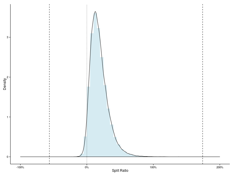
We can see that only a very small fraction of the field achieves a negative split. And that these runners generally only shave a few percent off their first half times. The dashed lines on the plot indicate the extreme values of the split ratio. Both of these are a long way from the body of the distribution. In statistical terms, either of these extremes is highly improbable.
If we categorise the runners broadly by the number of hours required to finish the race then we get a slightly different view of the data.
split.ratio = transform(split.ratio,
                        ihour = factor(floor(race.time / 60)))
levels(split.ratio$ihour) = sprintf("%s hour", levels(split.ratio$ihour))
#
(split.ratio.range = ddply(split.ratio, .(ihour), summarize, min = min(ratio), max = max(ratio)))
    ihour       min     max
1  5 hour -0.061526 0.24595
2  6 hour -0.130848 0.57918
3  7 hour -0.172256 0.84996
4  8 hour -0.563642 1.43530
5  9 hour -0.352379 1.46969
6 10 hour -0.270929 1.67596
7 11 hour -0.115299 1.74168
Runners who finish the race in less than 6 hours (in the “5 hour” bin above, which includes the race winner) have split ratios between -0.061526 and 0.24595. The 8 hour bin has ratios which range from -0.563642 to 1.43530. There was a runner in this group who was twice as fast in the second half… The 9 and 10 hour bins also have some inordinately large negative splits.
What about the distribution of splits in each of these categories?
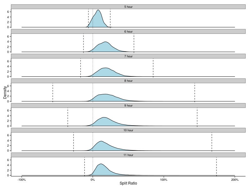
Now that paints an interesting picture. We can clearly see that in the 5 hour bin quite a significant proportion of the elite runners manage to achieve negative splits. The proportion in all the other bins is appreciably smaller, yet the extreme negative splits are very much larger!
Note that the density curve for the 5 hour bin extends slightly beyond the dashed line indicating the smallest value in this group. This is an artifact of the kernel density method used to create these curves, for which there is a trade off between the smoothness of the curve and the fidelity of the curve to the data. With a smoother curve the data are effectively smeared out more.
We can quantify those proportions.
negsplit.ihour = with(split.ratio, table(ihour, ratio < 0))
negsplit.ihour = negsplit.ihour / rowSums(negsplit.ihour)
#
negsplit.ihour[,2] * 100
 5 hour  6 hour  7 hour  8 hour  9 hour 10 hour 11 hour
14.2857  2.8740  2.2335  3.0653  3.1862  3.8505  1.9485
Around 14.3% of the runners in the 5 hour bin shave off some time in the second half of the race. In the other bins only around 2% to 3% of runners manage to achieve this feat.
Finally, before we dig into the details of some individual runners, let’s see how things vary from year to year.
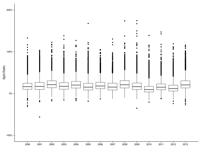
These data are more or less consistent between years. The median of the ratio is around 10% to 20%; the maximum is always roughly 100% or more; the minimum fluctuates rather wildly, extending from the credible -9.7% all the way down to the incredible -56.4%
ddply(split.ratio, .(year), summarize, median = median(ratio), min = min(ratio), max = max(ratio))
   year   median       min    max
1  2000 0.163330 -0.310556 1.3282
2  2001 0.168550 -0.563642 1.0321
3  2002 0.211599 -0.175799 1.2257
4  2003 0.171931 -0.151615 1.3793
5  2004 0.201743 -0.172256 1.2693
6  2005 0.151614 -0.183591 1.6760
7  2006 0.179430 -0.131274 1.0500
8  2007 0.153102 -0.129477 1.3033
9  2008 0.208643 -0.096563 1.7379
10 2009 0.163242 -0.352379 1.7417
11 2010 0.093532 -0.206322 1.3878
12 2011 0.150365 -0.125141 1.4697
13 2012 0.118362 -0.240859 1.1876
14 2013 0.204870 -0.270929 1.1596
Individual Runners
We are going to focus our attention on those runners with suspiciously large negative splits. These have been identified on the plot below as those with ratios less than -15% (that is, to the left of the dotted line). The threshold at -15% is somewhat arbitrary, but is certainly conservative.
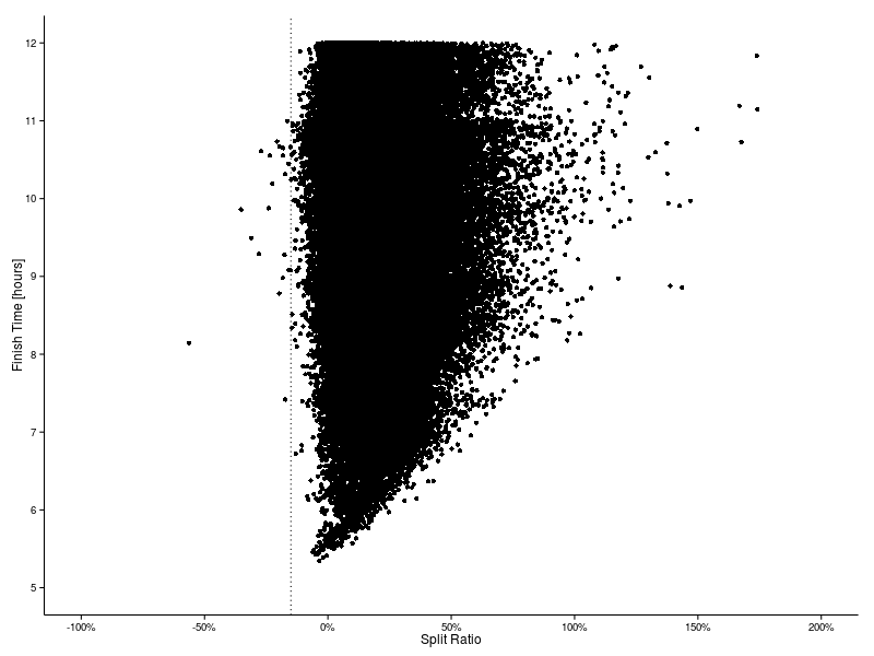
We extract only those records with ratios less than -15% and discard fields (like race number) to enforce a degree of anonymity. We will also add in a field to indicate how many times a runner appears in the list.
suspect = subset(split.ratio, ratio < RMIN)[, c("year", "key", "race.time", "ratio")]
(suspect = ddply(suspect, .(key), mutate, entries = length(ratio)))
   year      key race.time    ratio entries
1  2000 12bade96    545.20 -0.15863       1
2  2000 18e59575    557.25 -0.28027       1
3  2001 1a605ce5    488.82 -0.56364       1
4  2002 2edeb04e    556.53 -0.17580       1
5  2009 3c0ea3bc    591.63 -0.35238       2
6  2013 3c0ea3bc    636.50 -0.27093       2
7  2001   4abfd3    526.87 -0.19741       1
8  2013 4d5a86d7    659.88 -0.16419       1
9  2013 5cd624eb    640.05 -0.19636       1
10 2004 5ec9a72b    445.12 -0.17226       1
11 2012 7889f60a    592.57 -0.24086       1
12 2005  81f2015    538.72 -0.18359       1
13 2010 9f83c1a5    639.75 -0.15252       1
14 2003 a229ca86    544.75 -0.15161       1
15 2012 a59982c4    633.30 -0.18235       1
16 2010 a962c295    644.05 -0.20632       1
17 2010 ab59fc97    626.78 -0.15986       1
18 2001 c293e8f5    618.82 -0.17395       1
19 2013 e22d8c74    633.17 -0.23630       1
20 2000 ef35f2e6    569.48 -0.31056       1
21 2000 efdaf288    611.33 -0.22502       1
22 2005 fce308d5    638.98 -0.18083       1
That’s interesting, only one runner (the same guy with key 3c0ea3bc) appears twice.
We can take a look at the recent race history for these runners.
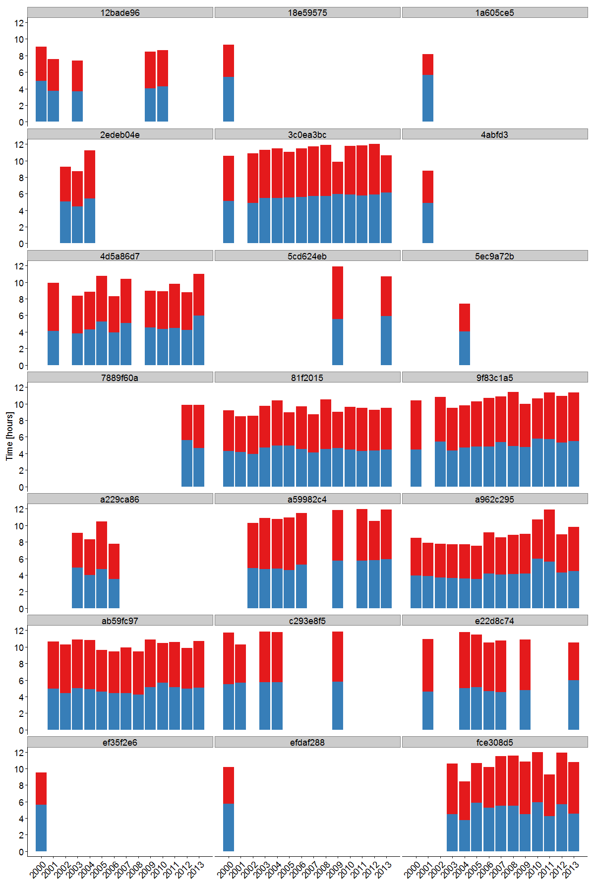
For a number of these runners there are only splits data for a few years, so it’s quite difficult to say anything conclusive. The negative split achieved by 1a605ce5 in 2001 looks pretty extreme though… Others runners, like 4d5a86d7, 9f83c1a5 and fce308d5 have a high degree of variability in both their first and second half times, so again it is difficult to spot an anomaly with certainty.
Let’s have a good look at 3c0ea3bc though. He has run the race consistently from 1991 to 2013. He did not finish in 1991 or 1997, but in the other years has managed to rack up 11 Bronze medals and 9 Vic Clapham medals, and in the process earned a double green number. The plot shows that his time to half way has been gradually increasing over the years. Not surprising since we all slow down with age. His finish time has mostly followed the same trend. Except for two major hiccups in 2009 and 2013. It’s hard to say for certain that these unusual negative splits were the result of cheating. But, equally, it’s hard to imagine how else they might have happened.
Here are the splits data for 3c0ea3bc:
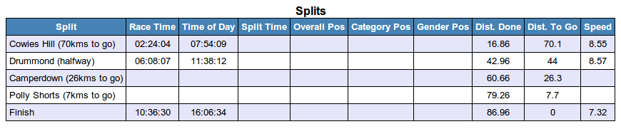
He was not recorded by either of the timing mats at Camperdown or Polly Shortts. It is well known that these mats are not perfect and sometimes they do miss runners. However, the missing splits at these mats plus the extraordinary time for the second half of the race are rather condemning.
I wonder what happened with those disciplinary hearings?