Following on from my previous post about Near Earth Objects, today we are going to solve Kepler’s Equation to find the eccentric anomaly, which is the next step towards plotting the positions of these NEOs relative to Earth.
The Eccentric, True and Mean Anomalies
The relationship between the eccentric and true anomalies are depicted in the figure below (courtesy of Wikipedia). We are thinking about the object located at P, which is moving along an elliptical orbit (the red curve). The true anomaly, $\theta$, is the angular position of P measured around the focus of the orbit (the location of the Sun in this case) relative to the direction of periapsis (the extension to the right of the line CF). The eccentric anomaly, E, is measured relative to the same line, but the angle is taken at the centre of the ellipse. The mean anomaly, M, does not have a direct geometric interpretation. Although it has a value between 0 and $2\pi $, it is not an angle. The mean anomaly relates position and time via Kepler’s Second Law, and is proportional to the area swept out by the line FP.

Kepler’s Equation
The eccentric anomaly, mean anomaly and orbit eccentricity are related by Kepler’s Equation:
$$ M = E - e \sin E. $$
This is a transcendental equation, meaning that it does not have an analytical solution. We will need to use numerical techniques to solve it.
Solving Kepler’s Equation
Recall that our NEO orbital data look like this:
head(orbits)
             Object Epoch        a         e          i         w     Node         M     q     Q    P    H     MOID class hazard
1  100004 (1983 VA) 56800 2.595899 0.6997035 0.28425360 0.2105033 1.349791 1.4094981 0.7795 4.41 4.18 16.4 0.176375   APO  FALSE
2 100085 (1992 UY4) 56800 2.639837 0.6248138 0.04892634 0.6689567 5.382550 0.2204248 0.9904 4.29 4.29 17.8 0.015111   APO   TRUE
3 100756 (1998 FM5) 56800 2.268602 0.5520201 0.20115638 5.4389541 3.086864 4.8250011 1.0163 3.52 3.42 16.1 0.100211   APO  FALSE
4  100926 (1998 MQ) 56800 1.782705 0.4077730 0.42286374 2.4205309 3.859910 3.4286821 1.0558 2.51 2.38 16.7 0.128731   AMO  FALSE
5  101869 (1999 MM) 56800 1.624303 0.6107117 0.08316718 4.6884786 1.938777 0.7584286 0.6323 2.62 2.07 19.3 0.001741   APO   TRUE
6 101873 (1999 NC5) 56800 2.029466 0.3933192 0.79884961 5.1531708 2.248914 5.6545349 1.2312 2.83 2.89 16.3 0.437678   AMO  FALSE
We are going to use the Newton-Raphson method via nleqslv() to solve Kepler’s Equation for each record.
library(nleqslv)
library(plyr)

# Solve Kepler's Equation to find the eccentric anomaly, E. This is a transcendental equation so we need to solve it
# numerically using the Newton-Raphson method.
#
orbits = ddply(orbits, .(Object), mutate, E = {
  kepler <- function(E) {
    M - E + e * sin(E)
  }

  nleqslv(0, kepler, method = "Newton")$x
})
head(orbits)[, c("Object", "E")]
             Object        E
1         (1979 XB) 5.632016
2         (1982 YA) 3.252744
3         (1983 LC) 2.280627
4         (1985 WA) 5.814292
5         (1986 NA) 2.591137
6        (1987 SF3) 5.268315
Plotting the Results
We will plot the resulting relationship between the mean and eccentric anomalies using colour to indicate eccentricity.
library(ggplot2)
library(scales)

degrees <- function(x, ...) {parse(text = paste0(x, "*degree"))}

ggplot(orbits, aes(x = M / pi * 180, y = E / pi * 180, colour = e)) +
  geom_point() +
  scale_colour_gradient("Eccentricity (e)", limits=c(0, 1), high = "red", low = "blue") +
  xlab("Mean Anomaly (M)") + ylab("Eccentric Anomaly (E)") +
  scale_x_continuous(labels = degrees, breaks = seq(0, 360, 90)) +
  scale_y_continuous(labels = degrees, breaks = seq(0, 360, 90)) +
  theme_classic()
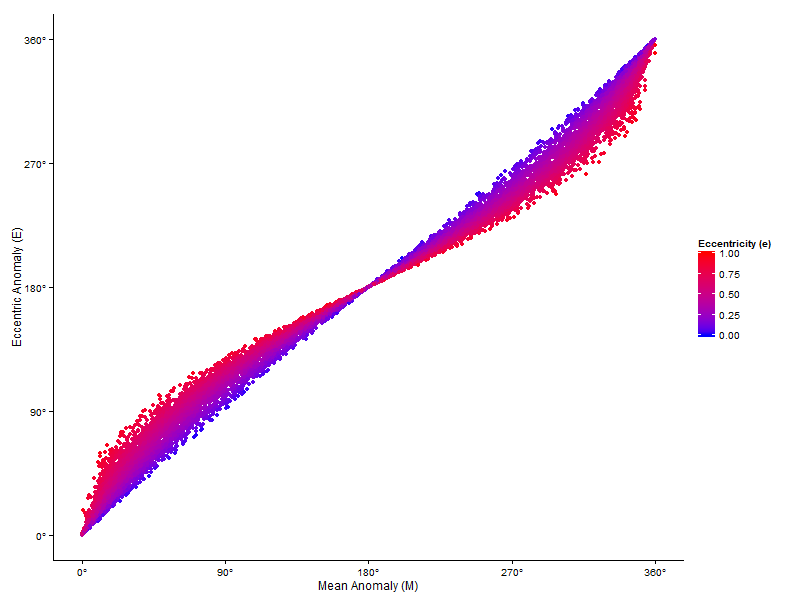
As one would expect, when the eccentricity is zero (a circular orbit) the relationship between the two anomalies is linear.
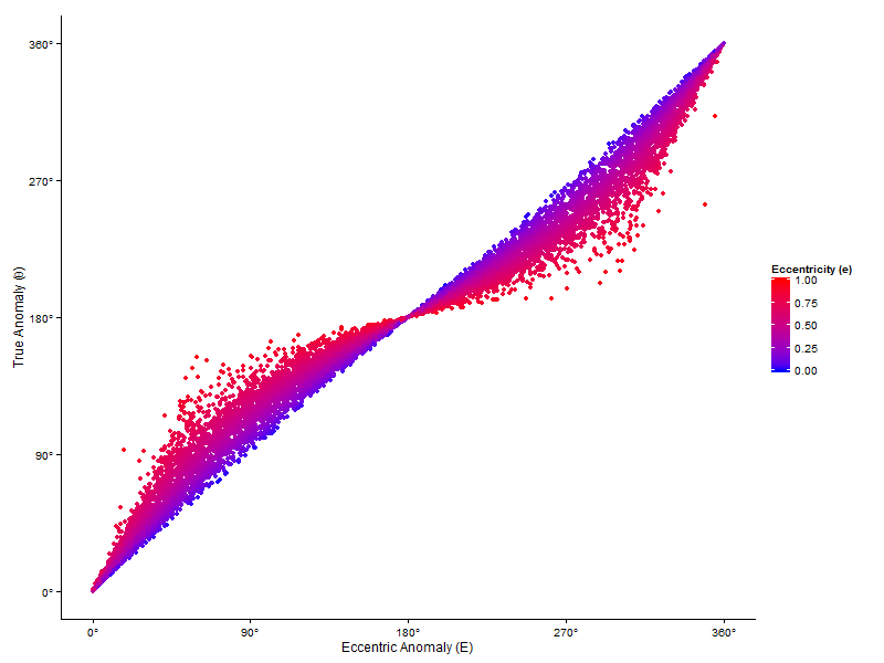
Finding the True Anomaly
Now it is a simple matter to get the true anomaly as well.
orbits = transform(orbits, theta = 2 * atan2(sqrt(1 + e) * sin (E/2), sqrt(1 - e) * cos (E/2)))
The Next Step
Now that we have the eccentric anomaly, we can calculate the Cartesian location of the objects in their respective orbital planes. We will then transform from the numerous orbital planes to a single reference frame.