Predicting Comrades Marathon finishing times is challenging and people have tried a few different approaches. Lindsey Parry, for example, suggests that you use two and a half times your recent marathon time. Sports Digest provides a calculator which predicts finishing time using recent times over three distances. I understand that this calculator is based on the work of Norrie Williamson.
Let’s give them a test. I finished the 2013 Comrades Marathon in 09:41. Based on my marathon time from February that year, which was 03:38, Parry’s formula suggests that I should have finished at around 09:07. Throwing in my Two Oceans time for that year, 04:59, and a 21.1 km time of 01:58 a few weeks before Comrades, the Sports Digest calculator gives a projected finish time of 08:59. Clearly, relative to both of those predictions, I under-performed that year! Either that or the predictions were way off the mark.
It seems to me that, given the volume of data we gather on our runs, we should be able to generate better predictions. If the thought of maths or data makes you want to doze off, feel free to jump ahead, otherwise read on.
Riegel’s Formula
In 1977 Peter Riegel published a formula for predicting running times, which became popular due to its simplicity. The formula itself looks like this:
$$ \Delta t_2 = \Delta t_1 \left( \frac{d_2}{d_1} \right)^{1.06} $$
which allows you to predict \(\Delta t_2\) the time it will take you to run distance \(d_2\), given that you know it takes you time \(\Delta t_1\) to run distance \(d_1\). Riegel called this his “endurance equation”.
Reverse-Engineering Riegel’s Model
Riegel’s formula is an empirical model: it’s based on data. In order to reverse engineer the model we are going to need some data too. Unfortunately I do not have access to data for a cohort of elite runners. However, I do have ample data for one particular runner: me. Since I come from the diametrically opposite end of the running spectrum (I believe the technical term would be “bog standard runner”), I think these data are probably more relevant to most runners anyway.
I compiled my data for the last three years based on the records kept by my trusty Garmin 910XT. A plot of time versus distance is given below.
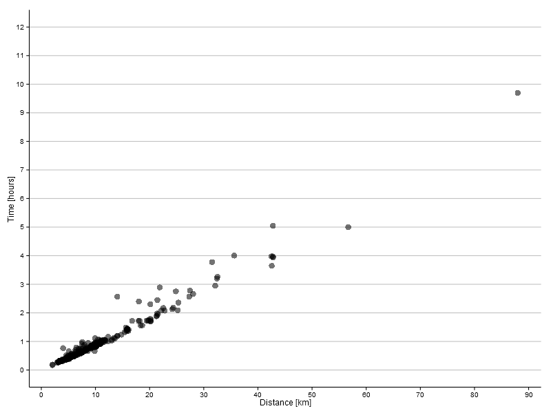
At first glance it looks like you could fit a straight line through those points. And you can, indeed, make a pretty decent linear fit.
> fit <- lm(TimeHours ~ Distance, data = training)
>
> summary(fit)

Call:
lm(formula = TimeHours ~ Distance, data = training)

Residuals:
     Min       1Q   Median       3Q      Max
-0.64254 -0.04592 -0.00618  0.02361  1.24900

Coefficients:
              Estimate Std. Error t value Pr(>|t|)
(Intercept) -0.1029964  0.0107648  -9.568   <2e-16 ***
Distance     0.1012847  0.0008664 116.902   <2e-16 ***
---
Signif. codes:  0 ‘***’ 0.001 ‘**’ 0.01 ‘*’ 0.05 ‘.’ 0.1 ‘ ’ 1

Residual standard error: 0.1394 on 442 degrees of freedom
Multiple R-squared:  0.9687,	Adjusted R-squared:  0.9686
F-statistic: 1.367e+04 on 1 and 442 DF,  p-value: < 2.2e-16
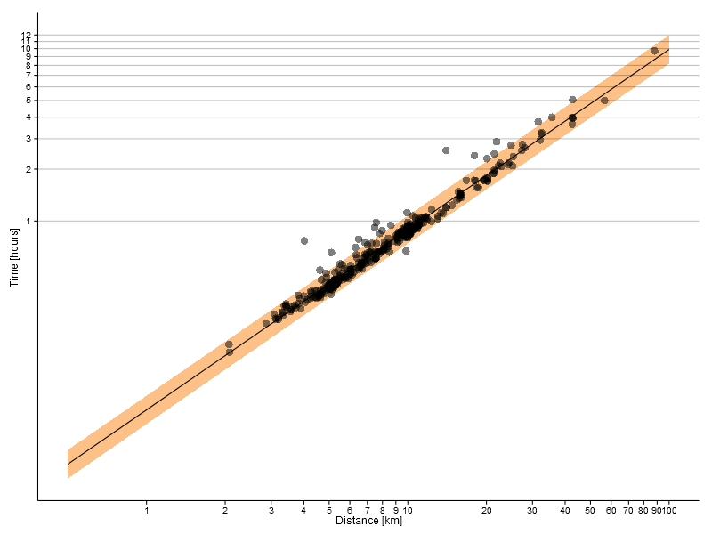
However, applying a logarithmic transform to both axes gives a more uniform distribution of the data, which also now looks more linear.
Riegel observed that data for a variety of disciplines (running, swimming, cycling and race walking) conformed to the same pattern. Figure 1 from this paper is included below.
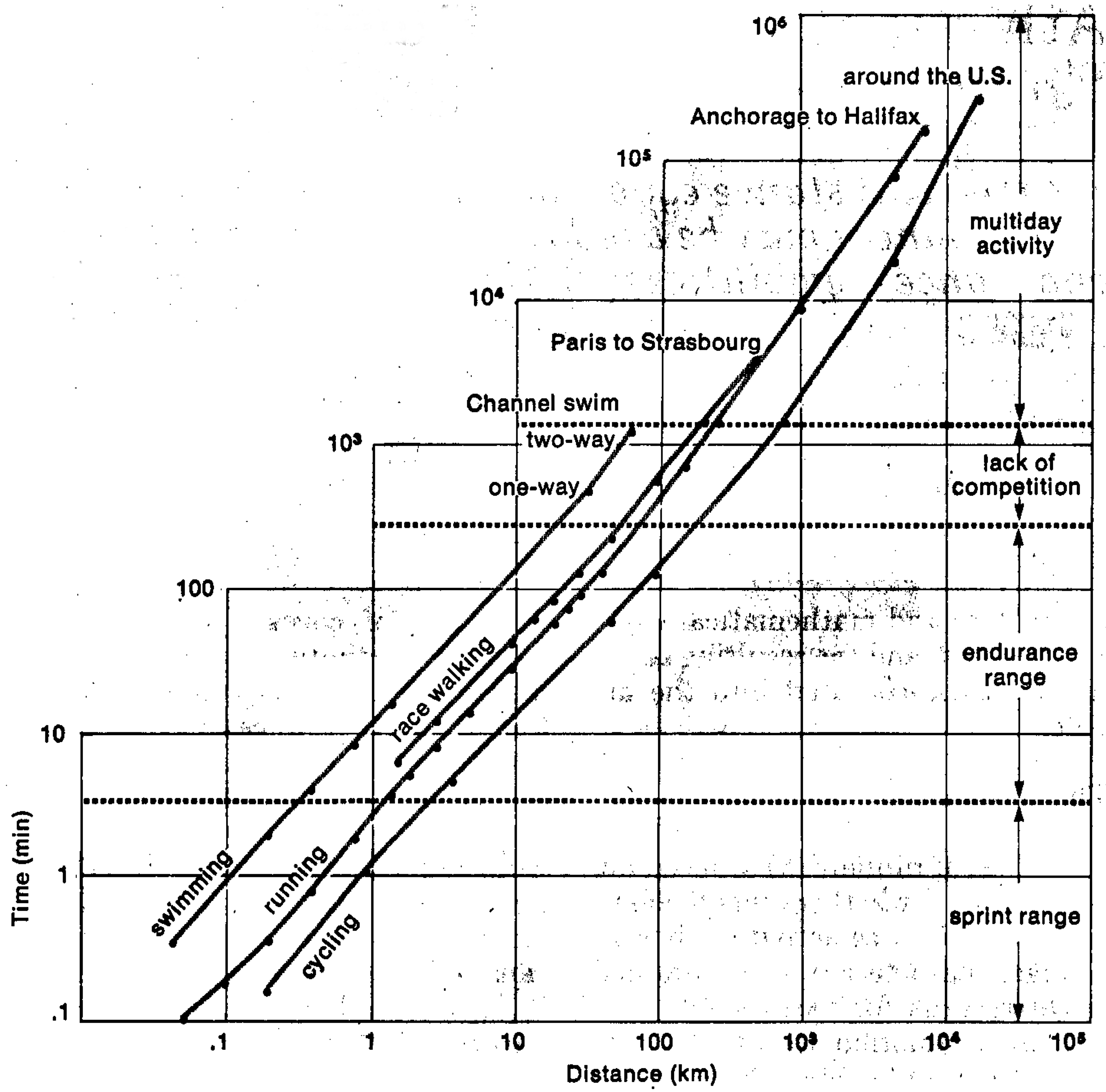
If we were to fit a straight line to the data on logarithmic axes then the relationship we’d be contemplating would have the form
$$\log \Delta t = m \log d + c$$
or, equivalently,
$$\Delta t = k d^m$$
which is a power law relating elapsed time to distance. It’s pretty easy to get Riegel’s formula from this. Taking two particular points on the power law, \(\Delta t_1 = k d_1^m\) and \(\Delta t_2 = k d_2^m\), and eliminating \(k\) gives
$$\Delta t_2 = \Delta t_2 \left( \frac{d_2}{d_1} \right)^m$$
which is Riegel’s formula with an unspecified value for the exponent. We’ll call the exponent the “fatigue factor” since it determines the degree to which a runner slows down as distance increases.
How do we get a value for the fatigue factor? Well, by fitting the data, of course!
> fit <- lm(log(TimeHours) ~ log(Distance), data = training)
>
> summary(fit)

Call:
lm(formula = log(TimeHours) ~ log(Distance), data = training)

Residuals:
     Min       1Q   Median       3Q      Max
-0.27095 -0.04809 -0.01843  0.01552  0.80351

Coefficients:
               Estimate Std. Error t value Pr(>|t|)
(Intercept)   -2.522669   0.018111  -139.3   <2e-16 ***
log(Distance)  1.045468   0.008307   125.9   <2e-16 ***
---
Signif. codes:  0 ‘***’ 0.001 ‘**’ 0.01 ‘*’ 0.05 ‘.’ 0.1 ‘ ’ 1

Residual standard error: 0.09424 on 442 degrees of freedom
Multiple R-squared:  0.9729,	Adjusted R-squared:  0.9728
F-statistic: 1.584e+04 on 1 and 442 DF,  p-value: < 2.2e-16
The fitted value for the exponent is 1.05 (rounding up), which is pretty close to the value in Riegel’s formula. The fitted model is included in the logarithmic plot above as the solid line, with the 95% prediction confidence interval indicated by the coloured ribbon. The linear plot below shows the data points used for training the model, the fit and confidence interval as well as dotted lines for constant paces ranging from 04:00 per km to 07:00 per km.
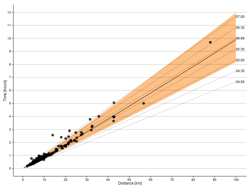
Our model also provides us with an indication of the uncertainty in the fitted exponent: the 95% confidence interval extends from 1.029 to 1.062.
> confint(fit)
                  2.5 %    97.5 %
(Intercept)   -2.558264 -2.487074
log(Distance)  1.029142  1.061794
Estimating the Fatigue Factor
A fatigue factor of 1 would correspond to a straight line, which implies a constant pace regardless of distance. A value less than 1 implies faster pace at larger distances (rather unlikely in practice). Finally, a value larger than 1 implies progressively slower pace at larger distances.
The problem with the fatigue factor estimate above, which was based on a single model fit to all of the data, is that it’s probably biased by the fact that most of the data are for runs of around 10 km. In this regime the relationship between time and distance is approximately linear, so that the resulting estimate of the fatigue factor is probably too small.
To get around this problem, I employed a bootstrap technique, creating a large number of subsets from the data. In each subset I weighted the samples to ensure that there was a more even distribution of distances in the mix. I calculated the fatigue factor for each subset, resulting in a range of estimates. Their distribution is plotted below.
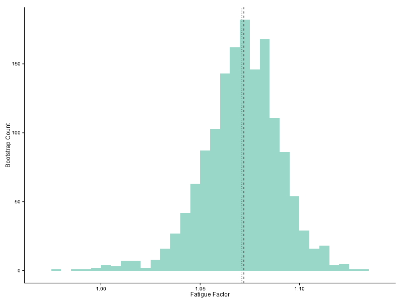
According to this analysis, my personal fatigue factor is around 1.07 (the median value indicated by the dashed line in the plot above). The Shapiro-Wilk test suggests that the data is sufficiently non-Normal to justify a non-parameteric estimate of the 95% confidence interval for the fatigue factor, which runs from 1.03 to 1.11.
> shapiro.test(fatigue.factor)

	Shapiro-Wilk normality test

data:  fatigue.factor
W = 0.9824, p-value = 1.435e-12

> median(fatigue.factor)
[1] 1.072006
> quantile(fatigue.factor, c(0.025, 0.975))
    2.5%    97.5%
1.030617 1.107044
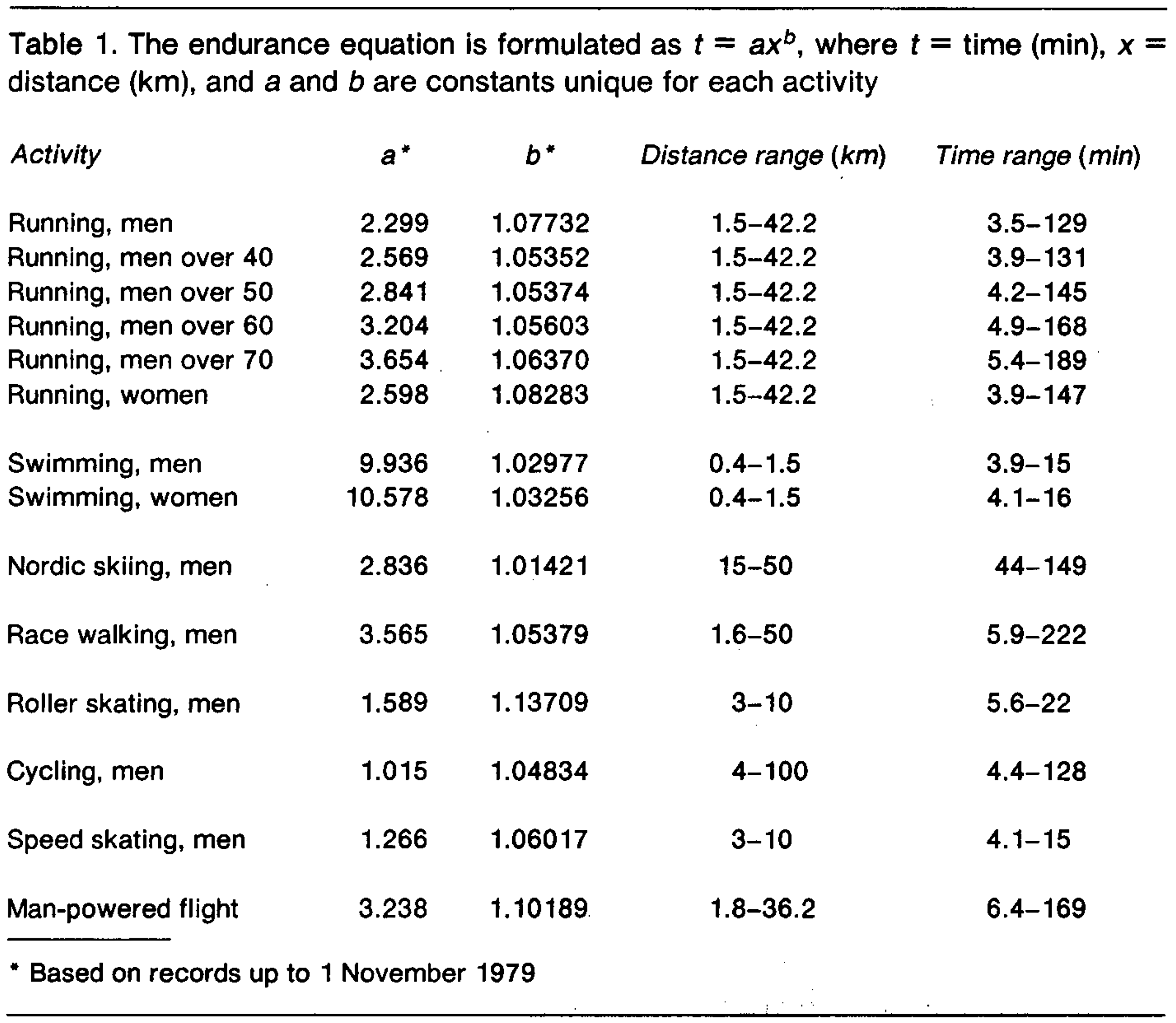
Riegel’s analysis also lead to a range of values for the fatigue factor. As can be seen from the table below (extracted from his paper), the values range from 1.01 for Nordic skiing to 1.14 for roller skating. Values for running range from 1.05 to 1.08 depending on age group and gender.
Generating Predictions
The rules mentioned above for predicting finishing times are generally applied to data for a single race (or a selection of three races). But, again, given that we have so much data on hand, would it not make sense to generate a larger set of predictions?
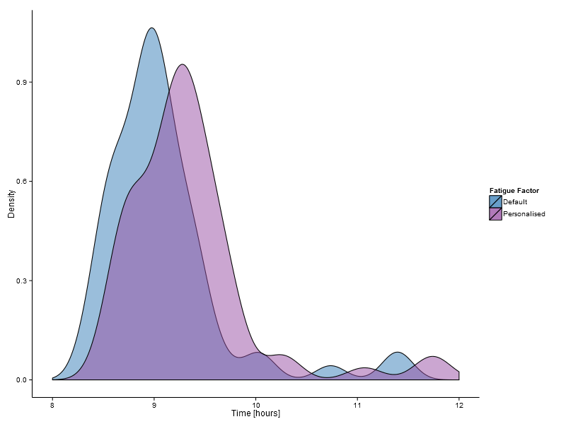
The distributions above indicate the predictions for this year’s Comrades Marathon (which is apparently going to be 89 km) based on all of my training data this year and using both the default (1.06) and personalised (1.07) values for the fatigue factor. The distributions are interesting, but what we are really interested in is the expected finish times, which are 08:59 and 09:18 depending on what value you use for the fatigue factor. I have a little more confidence in my personalised value, so I am going to be aiming for 09:18 this year.
Comrades is a long day and a variety of factors can affect your finish time. It’s good to have a ball-park idea though. If you would like me to generate a set of personalised predictions for you, just get in touch via the replies below.
Postscript
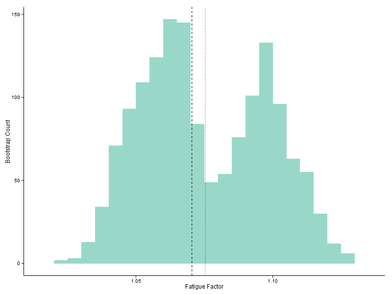
I repeated the analysis for one of my friends and colleagues. His fatigue factor also comes out as 1.07 although, interestingly, the distribution is bi-modal. I think I understand the reason for this though: his runs are divided clearly into two groups: training runs and short runs back and forth between work and the gym.
