An interesting paper (Modelling the recent common ancestry of all living humans, Nature, 431, 562–566, 2004) by Rohde, Olson and Chang concludes with the words:
Further work is needed to determine the effect of this common ancestry on patterns of genetic variation in structured populations. But to the extent that ancestry is considered in genealogical rather than genetic terms, our findings suggest a remarkable proposition: no matter the languages we speak or the colour of our skin, we share ancestors who planted rice on the banks of the Yangtze, who first domesticated horses on the steppes of the Ukraine, who hunted giant sloths in the forests of North and South America, and who laboured to build the Great Pyramid of Khufu.
This paper considered two models of our genealogical heritage. Neither of the models was exhaustive and they could not take into account all of the complexities involved in determining the genealogy of the Earth’s population. However, they captured many of the essential features. And despite their relative simplicity, the models reveal an unexpected result: a genealogical Common Ancestor (CA) of the entire present day human population would have lived in the relatively recent past.
It would be interesting to replicate some of those results.
An Even Simpler Model
In an earlier paper, Recent common ancestors of all present-day individuals, Chang considered a simpler model which he described as follows:
We assume the population size is constant at n. Generations are discrete and non-overlapping. The genealogy is formed by this random process: in each generation, each individual chooses two parents at random from the previous generation. The choices are made just as in the standard Wright–Fisher model (randomly and equally likely over the n possibilities) the only difference being that here each individual chooses twice instead of once. All choices are made independently. Thus, for example, it is possible that when an individual chooses his two parents, he chooses the same individual twice, so that in fact he ends up with just one parent; this happens with probability 1/n.
At first sight this appears to be an extremely crude and abstract model. However it captures many of the essential features required for modelling genealogical inheritance. It also has the advantage of not being too difficult to implement in R. If these details are not your cup of tea, feel free to skip forward to the results.
First we’ll need a couple of helper functions to neatly generate labels for generations (G) and individuals (I).
label.individuals <- function(N) {
   paste("I", str_pad(1:N, 2, pad = "0"), sep = "")
}

make.generation <- function(N, g) {
   paste(paste0("G", str_pad(g, 2, pad = "0")), label.individuals(N), sep = "/")
}

make.generation(3, 5)
[1] "G05/I01" "G05/I02" "G05/I03"
Each individual is identified by a label of the form “G05/I01”, which gives the generation number and also the specific identifier within that generation.
Next we’ll have a function to generate the random links between individuals in successive generations. The function will take two arguments: the number of individuals per generation and the number of ancestor generations (those prior to the “current” generation).
# N - number of people per generation
# G - number of ancestor generations (there will be G+1 generations!)
#
generate.edges <- function(N, G) {
   edges = lapply(0:(G-1),  function(g) {
     children <- rep(make.generation(N, g), each = 2)
     #
     parents <- sample(make.generation(N, g+1), 2 * N, replace = TRUE)
     #
     data.frame(parents = parents, children = children, stringsAsFactors = FALSE)
   })
   do.call(rbind, edges)
}

head(generate.edges(3, 3), 10)
   parents children
1  G01/I02  G00/I01
2  G01/I01  G00/I01
3  G01/I01  G00/I02
4  G01/I02  G00/I02
5  G01/I01  G00/I03
6  G01/I03  G00/I03
7  G02/I02  G01/I01
8  G02/I01  G01/I01
9  G02/I01  G01/I02
10 G02/I02  G01/I02
For example, the data generated above links the child node G00/I01 (individual 1 in generation 0) to two parent nodes, G01/I02 and G01/I01 (individuals 1 and 2 in generation 1).
Finally we’ll wrap all of that up in a graph-like object.
library(igraph)
  generate.nodes <- function(N, G) {
  lapply(0:G, function(g) make.generation(N, g))
}

generate.graph <- function(N, G) {
   nodes = generate.nodes(N, G)
   #
   net <- graph.data.frame(generate.edges(N, G), directed = TRUE, vertices = unlist(nodes))
   #
   # Edge layout
   #
   x = rep(1:N, G+1)
   y = rep(0:G, each = N)
   #
   net$layout = cbind(x, y)
   #
   net$individuals = label.individuals(N)
   net$generations = nodes
   #
   net
}
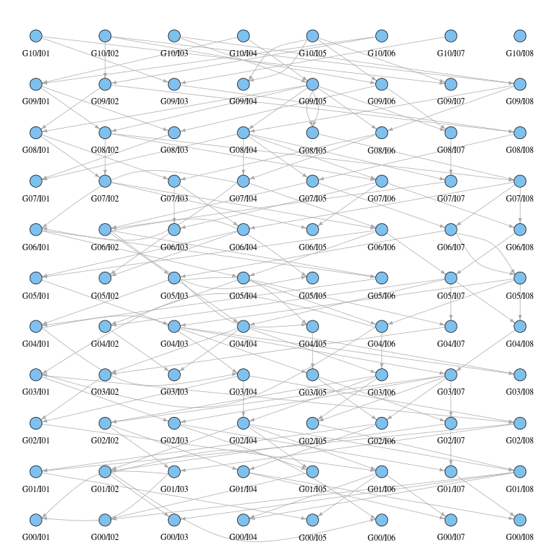
Let’s give it a whirl on a graph consisting of 10 ancestor generations (11 generations including the current generation) and 8 individuals per generation. The result is plotted below with the oldest generation (G10) at the top and the current generation (G00) at the bottom. The edges indicate parent/progeny links.
Okay, so it looks like all of the infrastructure is in place. Now we need to put together the functionality for analysing the relationships between generations. We are really only interested in how any one of the ancestor generations relates to the current generation, which makes things a little simpler. First we write a function to calculate the number of steps from an arbitrary node (identified by label) to each of the nodes in the current generation. This is simplified by the fact that igraph already has a shortest.path() function.
generation.descendants <- function(net, node) {
   present.generation <- first(net$generations)
   #
   shortest.paths(net, v = node, to = present.generation, mode = "out")
}
Next a pair of helper functions which indicate whether a particular node is a CA of all nodes in the current generation or if it has gone extinct. Node G03/I08 in the above graph is an example of an extinct node since it has no child nodes.
common.ancestor <- function(net, node) {
   all(is.finite(generation.descendants(net, node)))
}

extinct <- function(net, node) {
   all(is.infinite(generation.descendants(net, node)))
}
Let’s test those. We’ll generate another small graph for the test.
set.seed(1)
#
net <- generate.graph(3, 5)
#
# This is an ancestor of all.
#
generation.descendants(net, "G05/I01")
        G00/I01 G00/I02 G00/I03
G05/I01       5       5       5
> common.ancestor(net, "G05/I01")
[1] TRUE
# This is an ancestor of all but G00/I02
#
generation.descendants(net, "G02/I03")
        G00/I01 G00/I02 G00/I03
G02/I03       2     Inf       2
common.ancestor(net, "G02/I03")
[1] FALSE
# This node is extinct.
#
generation.descendants(net, "G03/I01")
        G00/I01 G00/I02 G00/I03
G03/I01     Inf     Inf     Inf
extinct(net, "G03/I01")
[1] TRUE
It would also be handy to have a function which gives the distance from every node in a particular generation to each of the nodes in the current generation.
generation.distance <- function(net, g) {
   current.generation <- net$generations[[g+1]]
   #
   do.call(rbind, lapply(current.generation, function(n) {generation.descendants(net, n)}))
}
generation.distance(net, 3)
        G00/I01 G00/I02 G00/I03
G03/I01     Inf     Inf     Inf
G03/I02       3       3       3
G03/I03       3       3       3
Here we see that G03/I02 and G03/I03 are both ancestors of each of the individuals in the current generation, while G03/I01 has gone extinct.
Finally we can pull all of this together with a single function that classifies individuals in previous generations according to whether they are an ancestor of at least one but not all of the current generation; a common ancestor of all of the current generation; or extinct.
classify.generation <- function(net, g) {
   factor(apply(generation.distance(net, g), 1, function(p) {
     ifelse(all(is.infinite(p)), 1, ifelse(all(is.finite(p)), 2, 0))
   }), levels = 0:2, labels = c("ancestor", "extinct", "common"))
}
classify.generation(net, 3)
G03/I01 G03/I02 G03/I03
extinct  common  common
Levels: ancestor extinct common
Results
First let’s have a look at how the relationship between previous generations and the current generation changes over time. The plot below indicates the proportion of ancestors, common ancestors and extinct individuals as a function of generation number. Note that time runs backwards along the horizontal axis, with the current generation on the left and successive ancestor generations moving towards the right.
The graph used to generate these data had 1000 individuals per generation. We can see that for the first 10 generations around 80% of the individuals were ancestors of one or more (but not all!) of the current generation. The remaining 20% or so were extinct. Then in generation 11 we have the first CA. This individual would be labelled the Most Recent Common Ancestor (MRCA). Going further back in time the fraction of CAs increases while the proportion of mere ancestors declines until around generation 19 when all of the ancestors are CAs.
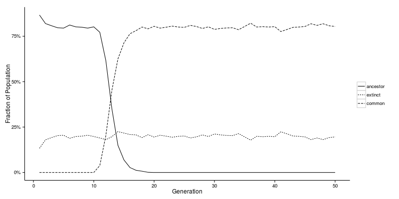
There are two important epochs to identify on the plot above:
- the generation at which the MRCA emerged (this is denoted \(T_n\)); and
- the generation at which all individuals are either CAs or extinct (this is denoted \(U_n\)).
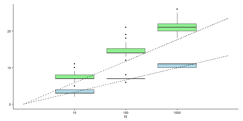
Chang’s paper gives asymptotic expressions for how these epochs vary as a function of generation size. It also presents a table with sample values of \(T_n\) and \(U_n\) for generations of size 500, 1000, 2000 and 4000. Those samples support the asymptotic relationships.
Since we have all of the infrastructure in place, we can conduct an independent test of the relationships. Below is a boxplot generated from 100 realisations each of calculations with generations of size 10, 100 and 1000. The blue boxes reflect our estimates for \(T_n\), while the green boxes are the estimates of \(U_n\). The two dashed lines reflect the asymptotic relationships. There’s pretty good agreement between the theoretical and experimental results, although our estimates for \(U_n\) appear to be consistently larger than expected. The sample size was limited though… Furthermore, these are asymptotic relationships, so we really only expect them to hold exactly for large generation sizes.
When would our MRCA have been alive based on this simple model and the Earth’s current population? Setting the generation size to the Earth’s current population of around 7 billion people gives \(T_n\) at about 33 generations and a \(U_n\) of approximately 58 generations. I know, those 7 billion people are not from the same generation, but we are going for an estimate here…
What does a generation translate to in terms of years? That figure has varied significantly over time. It also depends on location. However, in developed nations it is currently around 30 years. WolframAlpha equates a generation to 28 years. Based on these estimates we have \(T_n\) at around 1000 years and our estimate of \(U_n\) translates into less than 2 millennia.
Of course, these numbers need to be taken with a pinch of salt since they are based on a model which assumes that the population has been static at around 7 billion, which we know to be far from true! However these results are also not completely incompatible with the more sophisticated results of Rohde, Olson and Chang who found that the MRCA of all present-day humans lived just a few thousand years ago.