Sudoku-as-a-Service is a great illustration of Julia’s integer programming facilities. Julia has several packages which implement various flavours of optimisation: JuMP, JuMPeR, Gurobi, CPLEX, DReal, CoinOptServices and OptimPack. We’re not going to look at anything quite as elaborate as Sudoku today, but focus instead on finding the extrema in some simple (or perhaps not so simple) mathematical functions. At this point you might find it interesting to browse through this catalog of test functions for optimisation.
Optim
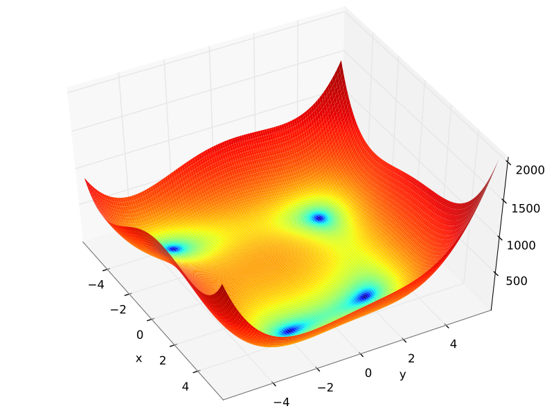
We’ll start out by using the Optim package to find extrema in Himmelblau’s function:
$$ f(x, y) = (x^2+y-11)^2 + (x+y^2-7)^2. $$
This function has one maximum and four minima. One of the minima is conveniently located at
$$ (x, y) = (3, 2). $$
As usual the first step is to load the required package.
using Optim
Then we set up the objective function along with its gradient and Hessian functions.
function himmelblau(x::Vector)
  (x[1]^2 + x[2] - 11)^2 + (x[1] + x[2]^2 - 7)^2
end
himmelblau (generic function with 1 method)
function himmelblau_gradient!(x::Vector, gradient::Vector)
  gradient[1] = 4 \* x[1] \* (x[1]^2 + x[2] - 11) + 2 * (x[1] + x[2]^2 - 7)
  gradient[2] = 2 \* (x[1]^2 + x[2] - 11) + 4 \* x[2] * (x[1] + x[2]^2 - 7)
end
himmelblau_gradient! (generic function with 1 method)
function himmelblau_hessian!(x::Vector, hessian::Matrix)
  hessian[1, 1] = 4 \* (x[1]^2 + x[2] - 11) + 8 \* x[1]^2 + 2
  hessian[1, 2] = 4 \* x[1] + 4 \* x[2]
  hessian[2, 1] = 4 \* x[1] + 4 \* x[2]
  hessian[2, 2] = 4 \* (x[1] + x[2]^2 - 7) + 8 \* x[2]^2 + 2
end
himmelblau_hessian! (generic function with 1 method)
There are a number of algorithms at our disposal. We’ll start with the Nelder Mead method which only uses the objective function itself. I am very happy with the detailed output provided by the optimize() function and clearly it converges on a result which is very close to what we expected.
optimize(himmelblau, [2.5, 2.5], method = :nelder_mead)
Results of Optimization Algorithm
 * Algorithm: Nelder-Mead
 * Starting Point: [2.5,2.5]
 * Minimum: [3.0000037281643586,2.0000105449945313]
 * Value of Function at Minimum: 0.000000
 * Iterations: 35
 * Convergence: true
   * |x - x'| < NaN: false
   * |f(x) - f(x')| / |f(x)| < 1.0e-08: true
   * |g(x)| < NaN: false
   * Exceeded Maximum Number of Iterations: false
 * Objective Function Calls: 69
 * Gradient Call: 0
Next we’ll look at the limited-memory version of the BFGS algorithm. This can be applied either with or without an explicit gradient function. In this case we’ll provide the gradient function defined above. Again we converge on the right result, but this time with far fewer iterations required.
optimize(himmelblau, himmelblau_gradient!, [2.5, 2.5], method = :l_bfgs)
Results of Optimization Algorithm
 * Algorithm: L-BFGS
 * Starting Point: [2.5,2.5]
 * Minimum: [2.999999999999385,2.0000000000001963]
 * Value of Function at Minimum: 0.000000
 * Iterations: 6
 * Convergence: true
   * |x - x'| < 1.0e-32: false
   * |f(x) - f(x')| / |f(x)| < 1.0e-08: false
   * |g(x)| < 1.0e-08: true
   * Exceeded Maximum Number of Iterations: false
 * Objective Function Calls: 25
 * Gradient Call: 25
Finally we’ll try out Newton’s method, where we’ll provide both gradient and Hessian functions. The result is spot on and we’ve shaved off one iteration. Very nice indeed!
optimize(himmelblau, himmelblau_gradient!, himmelblau_hessian!, [2.5, 2.5], method = :newton)
Results of Optimization Algorithm
 * Algorithm: Newton's Method
 * Starting Point: [2.5,2.5]
 * Minimum: [3.0,2.0]
 * Value of Function at Minimum: 0.000000
 * Iterations: 5
 * Convergence: true
   * |x - x'| < 1.0e-32: false
   * |f(x) - f(x')| / |f(x)| < 1.0e-08: true
   * |g(x)| < 1.0e-08: true
   * Exceeded Maximum Number of Iterations: false
 * Objective Function Calls: 19
 * Gradient Call: 19
There is also a Simulated Annealing solver in the Optim package.
NLopt
NLopt is an optimisation library with interfaces for a variety of programming languages. NLopt offers a variety of optimisation algorithms. We’ll apply both a gradient-based and a derivative-free technique to maximise the function
$$ \sin\alpha \cos\beta $$
subject to the constraints
$$ 2 \alpha \leq \beta $$
and
$$ \beta \leq \pi/2. $$
Before we load the NLopt package, it’s a good idea to restart your Julia session to flush out any remnants of the Optim package.
using NLopt
We’ll need to write the objective function and a generalised constraint function.
count = 0;
function objective(x::Vector, grad::Vector)
  if length(grad) > 0
    grad[1] = cos(x[1]) * cos(x[2])
    grad[2] = - sin(x[1]) * sin(x[2])
  end

  global count
  count::Int += 1
  println("Iteration $count: $x")

  sin(x[1]) * cos(x[2])
end
objective (generic function with 1 method)
function constraint(x::Vector, grad::Vector, a, b, c)
  if length(grad) > 0
    grad[1] = a
    grad[2] = b
  end
  a * x[1] + b * x[2] - c
end
constraint (generic function with 1 method)
The COBYLA (Constrained Optimization BY Linear Approximations) algorithm is a local optimiser which doesn’t use the gradient function.
opt = Opt(:LN_COBYLA, 2); 						# Algorithm and dimension of problem
ndims(opt)
2
algorithm(opt)
:LN_COBYLA
algorithm_name(opt) # Text description of algorithm
"COBYLA (Constrained Optimization BY Linear Approximations) (local, no-derivative)"
We impose generous upper and lower bounds on the solution space and use two inequality constraints. Either min_objective!() or max_objective!() is used to specify the objective function and whether or not it is a minimisation or maximisation problem. Constraints can be either inequalities using inequality_constraint!() or equalities using equality_constraint!().
lower_bounds!(opt, [0., 0.])
upper_bounds!(opt, [pi, pi])
xtol_rel!(opt, 1e-6)
max_objective!(opt, objective)
inequality_constraint!(opt, (x, g) -> constraint(x, g, 2, -1, 0), 1e-8)
inequality_constraint!(opt, (x, g) -> constraint(x, g, 0, 2, pi), 1e-8)
After making an initial guess we let the algorithm loose. I’ve purged some of the output to spare you from the floating point deluge.
initial = [0, 0]; 								# Initial guess
(maxf, maxx, ret) = optimize(opt, initial)
Iteration 1: [0.0,0.0]
Iteration 2: [0.7853981633974483,0.0]
Iteration 3: [0.7853981633974483,0.7853981633974483]
Iteration 4: [0.0,0.17884042066163552]
Iteration 5: [0.17562036827601815,0.3512407365520363]
Iteration 6: [0.5268611048280544,1.053722209656109]
Iteration 7: [0.7853981633974481,1.5707963267948961]
Iteration 8: [0.7526175675681757,0.9963866471510139]
Iteration 9: [0.785398163397448,1.570796326794896]
Iteration 10: [0.35124073655203625,0.7024814731040726]
.
.
.
Iteration 60: [0.42053333513020824,0.8410666702604165]
Iteration 61: [0.42053467500728553,0.8410693500145711]
Iteration 62: [0.4205360148843628,0.8410720297687256]
Iteration 63: [0.4205340050687469,0.8410680101374938]
Iteration 64: [0.4205340249920041,0.8410677994554656]
Iteration 65: [0.42053333513020824,0.8410666702604165]
Iteration 66: [0.42053456716611504,0.8410679945560181]
Iteration 67: [0.42053333513020824,0.8410666702604165]
Iteration 68: [0.42053365382801033,0.8410673076560207]
(0.27216552697496077,[0.420534,0.841067],:XTOL_REACHED)
println("got $maxf at $maxx after $count iterations.")
got 0.27216552697496077 at [0.42053365382801033,0.8410673076560207] after 68 iterations.
It takes a number of iterations to converge, but arrives at a solution which seems eminently reasonable (and which satisfies both of the constraints).
Next we’ll use the MMA (Method of Moving Asymptotes) gradient-based algorithm.
opt = Opt(:LD_MMA, 2);
We remove the second inequality constraint and simply confine the solution space appropriately. This is definitely a more efficient approach!
lower_bounds!(opt, [0., 0.])
upper_bounds!(opt, [pi, pi / 2])
xtol_rel!(opt, 1e-6)
max_objective!(opt, objective)
inequality_constraint!(opt, (x, g) -> constraint(x, g, 2, -1, 0), 1e-8)
This algorithm converges more rapidly (because it takes advantage of the gradient function!) and we arrive at the same result.
(maxf, maxx, ret) = optimize(opt, initial)
Iteration 1: [0.0,0.0]
Iteration 2: [0.046935706114911574,0.12952531487499092]
Iteration 3: [0.1734128499487191,0.5065804625164063]
Iteration 4: [0.3449211909390502,0.7904095832845456]
Iteration 5: [0.4109653874949588,0.8281977630709889]
Iteration 6: [0.41725447118163134,0.8345944447401356]
Iteration 7: [0.4188068871033356,0.8376261095301502]
Iteration 8: [0.4200799333613666,0.8401670014914709]
Iteration 9: [0.4203495290598476,0.8406993867808531]
Iteration 10: [0.4205138682235357,0.8410278412850836]
Iteration 11: [0.4205289336960578,0.8410578710185219]
Iteration 12: [0.42053231747822034,0.8410646372592685]
Iteration 13: [0.42053444274035756,0.8410688833806734]
Iteration 14: [0.4205343574933894,0.8410687141629858]
Iteration 15: [0.4205343707980632,0.8410687434944638]
Iteration 16: [0.420534312041705,0.8410686169530415]
Iteration 17: [0.4205343317839936,0.8410686604482764]
Iteration 18: [0.42053433111342814,0.8410686565253115]
Iteration 19: [0.42053433035398824,0.8410686525997696]
(0.27216552944315736,[0.420534,0.841069],:XTOL_REACHED)
println("got $maxf at $maxx after $count iterations.")
got 0.27216552944315736 at [0.42053433035398824,0.8410686525997696] after 19 iterations.
I’m rather impressed. Both of these packages provide convenient interfaces and I could solve my test problems without too much effort. Have a look at the videos below for more about optimisation in Julia and check out GitHub for the complete code for today’s examples. We’ll kick off next week with a quick look at some alternative data structures.
