Today I’m looking at the Distributions package.
Let’s get things rolling by loading it up.
using Distributions
There’s some overlap between the functionality in Distributions and what we saw yesterday in the StatsFuns package. Instead of looking at functions to evaluate various aspects of PDFs and CDFs, we’ll focus on sampling from distributions and calculating summary statistics.
Julia has native support for sampling from a uniform distribution. We’ve seen this before, but here’s a reminder.
srand(359) # Set random number seed.
rand() # Random number on [0, 1)
0.4770241944535658
What if you need to generate samples from a more exotic distribution? The Normal distribution, although not particularly exotic, seems like a natural place to start. The Distributions package exposes a type for each supported distribution. For the Normal distribution the type is appropriately named Normal. It’s derived from Distribution with characteristics Univariate and Continuous.
super(Normal)
Distribution{Univariate,Continuous}
names(Normal)
2-element Array{Symbol,1}:
 :μ
 :σ
The constructor accepts two parameters: mean (μ) and standard deviation (σ). We’ll instantiate a Normal object with mean 1 and standard deviation 3.
d1 = Normal(1.0, 3.0)
Normal(μ=1.0, σ=3.0)
params(d1)
(1.0,3.0)
d1.μ
1.0
d1.σ
3.0
Thanks to the wonders of multiple dispatch we are then able to generate samples from this object with the rand() method.
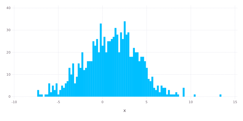
x = rand(d1, 1000);
We’ll use Gadfly to generate a histogram to validate that the samples are reasonable. They look pretty good.
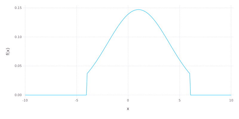
There are functions like pdf(), cdf(), logpdf() and logcdf() which allow the density function of our distribution object to be evaluated at particular points. Check those out. We’re moving on to truncating a portion of the distribution, leaving a Truncated distribution object.
d2 = Truncated(d1, -4.0, 6.0);
Again we can use Gadfly to get an idea of what this looks like. This time we’ll plot the actual PDF rather than a histogram of samples.
The Distributions package implements an extensive selection of other continuous distributions, like Exponential, Poisson, Gamma and Weibull. The basic interface for each of these is consistent with what we’ve seen for Normal above, although there are some methods which are specific to some distributions.
Let’s look at a discrete distribution, using a Bernoulli distribution with success rate of 25% as an example.
d4 = Bernoulli(0.25)
Bernoulli(p=0.25)
rand(d4, 10)
10-element Array{Int64,1}:
 0
 1
 0
 1
 1
 0
 0
 0
 1
 0
What about a Binomial distribution? Suppose that we have a success rate of 25% per trial and want to sample the number of successes in a batch of 100 trials.
d5 = Binomial(100, 0.25)
Binomial(n=100, p=0.25)
rand(d5, 10)
10-element Array{Int64,1}:
 22
 21
 30
 23
 28
 25
 26
 26
 28
 21
Finally let’s look at an example of fitting a distribution to a collection of samples using Maximum Likelihood.
x = rand(d1, 10000);
fit(Normal, x)
Normal(μ=1.0015796782177036, σ=3.033914550184868)
Yup, those values are in pretty good agreement with the mean and standard deviation we specified for our Normal object originally.
That’s it for today. There’s more to the Distributions package though. Check out my GitHub repository to see other examples which didn’t make it into the today’s post.