Today we’ll be looking at the Distances package, which implements a range of distance metrics. This might seem a rather obscure topic, but distance calculation is at the core of all clustering techniques (which are next on the agenda), so it’s prudent to know a little about how they work.
Note that there is a Distance package as well (singular!), which was deprecated in favour of the Distances package. Please install and load the latter.
using Distances
We’ll start by finding the distance between a pair of vectors.
x = [1., 2., 3.];
y = [-1., 3., 5.];
A simple application of Pythagoras’ Theorem will tell you that the Euclidean distance between the tips of those vectors is 3. We can confirm our maths with Julia though. The general form of a distance calculation uses evaluate(), where the first argument is a distance type. Common distance metrics (like Euclidean distance) also come with convenience functions.
evaluate(Euclidean(), x, y)
3.0
euclidean(x, y)
3.0
We can just as easily calculate other metrics like the city block (or Manhattan), cosine or Chebyshev distances.
evaluate(Cityblock(), x, y)
5.0
cityblock(x, y)
5.0
evaluate(CosineDist(), x, y)
0.09649209709474871
evaluate(Chebyshev(), x, y)
2.0
Moving on to distances between the columns of matrices. Again we’ll define a pair of matrices for illustration.
X = [0 1; 0 2; 0 3];
Y = [1 -1; 1 3; 1 5];
With colwise() distances are calculated between corresponding columns in the two matrices. If one of the matrices has only a single column (see the example with Chebyshev() below) then the distance is calculated between that column and all columns in the other matrix.
colwise(Euclidean(), X, Y)
2-element Array{Float64,1}:
 1.73205
 3.0
colwise(Hamming(), X, Y)
2-element Array{Int64,1}:
 3
 3
colwise(Chebyshev(), X[:,1], Y)
2-element Array{Float64,1}:
 1.0
 5.0
We also have the option of using pairwise() which gives the distances between all pairs of columns from the two matrices. This is precisely the distance matrix that we would use for a cluster analysis.
pairwise(Euclidean(), X, Y)
2x2 Array{Float64,2}:
 1.73205 5.91608
 2.23607 3.0
pairwise(Euclidean(), X)
2x2 Array{Float64,2}:
 0.0 3.74166
 3.74166 0.0
pairwise(Mahalanobis(eye(3)), X, Y) # Effectively just the Euclidean metric
2x2 Array{Float64,2}:
 1.73205 5.91608
 2.23607 3.0
pairwise(WeightedEuclidean([1.0, 2.0, 3.0]), X, Y)
2x2 Array{Float64,2}:
 2.44949 9.69536
 3.74166 4.24264
As you might have observed from the last example above, it’s also possible to calculate weighted versions of some of the metrics.
Finally a less contrived example. We’ll look at the distances between observations in the iris data set. We first need to extract only the numeric component of each record and then transpose the resulting matrix so that observations become columns (rather than rows).
using RDatasets
iris = dataset("datasets", "iris");
iris = convert(Array, iris[:,1:4]);
iris = transpose(iris);
dist_iris = pairwise(Euclidean(), iris);
dist_iris[1:5,1:5]
5x5 Array{Float64,2}:
 0.0 0.538516 0.509902 0.648074 0.141421
 0.538516 0.0 0.3 0.331662 0.608276
 0.509902 0.3 0.0 0.244949 0.509902
 0.648074 0.331662 0.244949 0.0 0.648074
 0.141421 0.608276 0.509902 0.648074 0.0
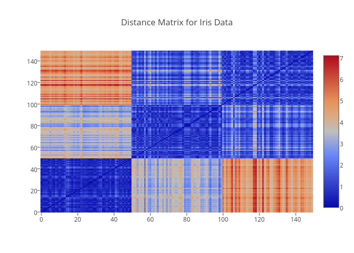
The full distance matrix is illustrated below as a heatmap using Plotly. Note how the clearly define blocks for each of the iris species Setosa, Versicolor, and Virginica.

Tomorrow we’ll be back to look at clustering in Julia.