Today we’ll be looking at two packages for regression analyses in Julia: GLM and GLMNet. Let’s get both of those loaded so that we can begin.
using GLM, GLMNet
Next we’ll create a synthetic data set which we’ll use for illustration purposes.
using Distributions, DataFrames
points = DataFrame();
points[:x] = rand(Uniform(0.0, 10.0), 500);
points[:y] = 2 + 3 * points[:x] + rand(Normal(1.0, 3.0) , 500);
points[:z] = rand(Uniform(0.0, 10.0), 500);
points[:valid] = 2 * points[:y] + points[:z] + rand(Normal(0.0, 3.0), 500) .> 35;
head(points)
6x4 DataFrame
| Row | x        | y       | z       | valid |
|-----|----------|---------|---------|-------|
| 1   | 0.867859 | 3.08688 | 6.03142 | false |
| 2   | 9.92178  | 33.4759 | 2.14742 | true  |
| 3   | 8.54372  | 32.2662 | 8.86289 | true  |
| 4   | 9.69646  | 35.5689 | 8.83644 | true  |
| 5   | 4.02686  | 12.4154 | 2.75854 | false |
| 6   | 6.89605  | 27.1884 | 6.10983 | true  |
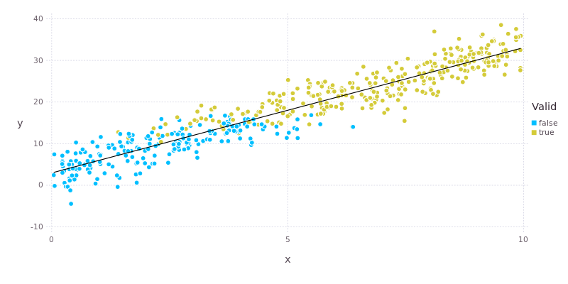
By design there is a linear relationship between the x and y fields. We can extract that relationship from the data using glm().
model = glm(y ~ x, points, Normal(), IdentityLink())
DataFrameRegressionModel{GeneralizedLinearModel{GlmResp{Array{Float64,1},Normal,IdentityLink},
                         DensePredChol{Float64,Cholesky{Float64}}},Float64}:

Coefficients:
             Estimate Std.Error z value Pr(>|z|)
(Intercept)   2.69863  0.265687 10.1572   <1e-23
x             2.99845 0.0474285 63.2204   <1e-99
The third and forth arguments to glm() stipulate that we are applying simple linear regression where we expect the residuals to have a Normal distribution. The parameter estimates are close to what was expected, taking into account the additive noise introduced into the data. The call to glm() seems rather verbose for something as simple as linear regression and, consequently, there is a shortcut lm() which gets the same result with less fuss.
Using the result of glm() we can directly access the estimated coefficients along with their standard errors and the associated covariance matrix.
coef(model)
2-element Array{Float64,1}:
 2.69863
 2.99845
stderr(model)
2-element Array{Float64,1}:
 0.265687
 0.0474285
vcov(model)
2x2 Array{Float64,2}:
  0.0705897  -0.0107768
 -0.0107768   0.00224947
The data along with the linear regression fit are shown below.

Moving on to the GLMNet package, which implements linear models with penalised maximum likelihood estimators. We’ll use the Boston housing data from R’s MASS package for illustration.
using RDatasets
boston = dataset("MASS", "Boston");
X = array(boston[:,1:13]);
y = array(boston[:,14]); # Median value of houses in units of $1000
Running glmnet() which will fit models for various values of the regularisation parameter, λ.
path = glmnet(X, y);
The result is a set of 76 different models. We’ll have a look at the intercepts and coefficients for the first ten models (which correspond to the largest values of λ). The coefficients are held in the betas field, which is an array with a column for each model and a row for each coefficient. Since the first few models are strongly penalised, each has only a few non-zero coefficients.
path.a0[1:10]
10-element Array{Float64,1}:
22.5328
23.6007
23.6726
21.4465
19.4206
17.5746
15.8927
14.3602
12.9638
12.5562
path.betas[:,1:10]
13x10 Array{Float64,2}:
 0.0  0.0        0.0       0.0       0.0       0.0       0.0       0.0       0.0      0.0
 0.0  0.0        0.0       0.0       0.0       0.0       0.0       0.0       0.0      0.0
 0.0  0.0        0.0       0.0       0.0       0.0       0.0       0.0       0.0      0.0
 0.0  0.0        0.0       0.0       0.0       0.0       0.0       0.0       0.0      0.0
 0.0  0.0        0.0       0.0       0.0       0.0       0.0       0.0       0.0      0.0
 0.0  0.0        0.127841  0.569442  0.971462  1.33777   1.67153   1.97564   2.25274  2.47954
 0.0  0.0        0.0       0.0       0.0       0.0       0.0       0.0       0.0      0.0
 0.0  0.0        0.0       0.0       0.0       0.0       0.0       0.0       0.0      0.0
 0.0  0.0        0.0       0.0       0.0       0.0       0.0       0.0       0.0      0.0
 0.0  0.0        0.0       0.0       0.0       0.0       0.0       0.0       0.0      0.0
 0.0  0.0        0.0       0.0       0.0       0.0       0.0       0.0       0.0     -0.040168
 0.0  0.0        0.0       0.0       0.0       0.0       0.0       0.0       0.0      0.0
 0.0 -0.0843998 -0.153581 -0.196981 -0.236547 -0.272599 -0.305447 -0.335377 -0.36264 -0.384493
Now that we’ve got a bundle of models, how do we choose among them? Cross-validation, of course!
path = glmnetcv(X, y)
Least Squares GLMNet Cross Validation
76 models for 13 predictors in 10 folds
Best λ 0.028 (mean loss 24.161, std 3.019)
We find that the best results (on the basis of loss) were achieved when λ had a value of 0.028, which is relatively weak regularisation. We’ll put the parameters of the corresponding model neatly in a data frame.
DataFrame(variable = names(boston)[1:13], beta = path.path.betas[:,indmin(path.meanloss)])
13x2 DataFrame
| Row | variable | beta       |
|-----|----------|------------|
| 1   | Crim     | -0.0983463 |
| 2   | Zn       | 0.0414416  |
| 3   | Indus    | 0.0        |
| 4   | Chas     | 2.68519    |
| 5   | NOx      | -16.3066   |
| 6   | Rm       | 3.86694    |
| 7   | Age      | 0.0        |
| 8   | Dis      | -1.39602   |
| 9   | Rad      | 0.252687   |
| 10  | Tax      | -0.0098268 |
| 11  | PTRatio  | -0.929989  |
| 12  | Black    | 0.00902588 |
| 13  | LStat    | -0.5225    |
From the fit coefficients we can conclude, for example, that average house value increases with the number of rooms in the house (Rm) but decreases with nitrogen oxides concentration (NOx), which is a proxy for traffic intensity.
Whew! That was exhilarating but exhausting. As a footnote, please have a look at the thesis “RegTools: A Julia Package for Assisting Regression Analysis” by Muzhou Liang. The RegTools package is available here. As always, the full code for today is available on github. Next time we’ll look at classification models. Below are a couple of pertinent videos to keep you busy in the meantime.