Yesterday we had a look at Julia’s regression model capabilities. A natural counterpart to these are models which perform classification. We’ll be looking at the GLM and DecisionTree packages. But, before I move on to that, I should mention the MLBase package which provides a load of functionality for data preprocessing, performance evaluation, cross-validation and model tuning.
Logistic Regression
Logistic regression lies on the border between the regression techniques we considered yesterday and the classification techniques we’re looking at today. In effect though it’s really a classification technique. We’ll use some data generated in yesterday’s post to illustrate. Specifically we’ll look at the relationship between the Boolean field valid and the three numeric fields.
head(points)
6x4 DataFrame
| Row | x        | y       | z       | valid |
|-----|----------|---------|---------|-------|
| 1   | 0.867859 | 3.08688 | 6.03142 | false |
| 2   | 9.92178  | 33.4759 | 2.14742 | true  |
| 3   | 8.54372  | 32.2662 | 8.86289 | true  |
| 4   | 9.69646  | 35.5689 | 8.83644 | true  |
| 5   | 4.02686  | 12.4154 | 2.75854 | false |
| 6   | 6.89605  | 27.1884 | 6.10983 | true  |
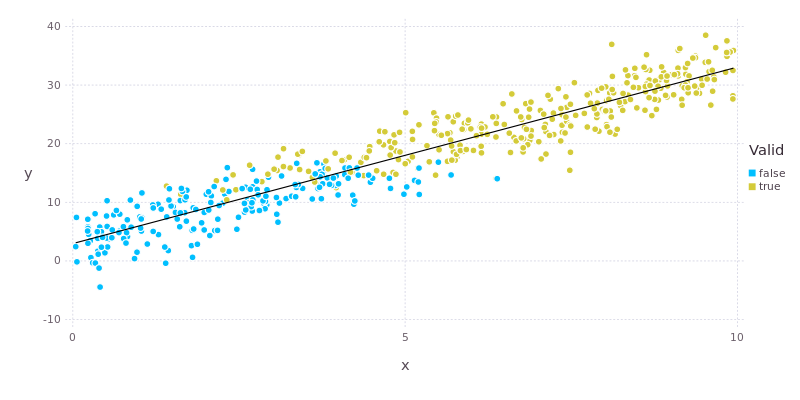
To further refresh your memory, the plot below shows the relationship between valid and the variables x and y. We’re going to attempt to capture this relationship in our model.

Logistic regression is also applied with the glm() function from the GLM package. The call looks very similar to the one used for linear regression except that the error family is now Binomial() and we’re using a logit link function.
model = glm(valid ~ x + y + z, points, Binomial(), LogitLink())
DataFrameRegressionModel{GeneralizedLinearModel{GlmResp{Array{Float64,1},Binomial,LogitLink},
                         DensePredChol{Float64,Cholesky{Float64}}},Float64}:
Coefficients:
              Estimate Std.Error   z value Pr(>|z|)
(Intercept)   -23.1457   3.74348  -6.18295    <1e-9
x            -0.260122  0.269059 -0.966786   0.3337
y              1.36143  0.244123    5.5768    <1e-7
z             0.723107   0.14739   4.90606    <1e-6
According to the model there is a significant relationship between valid and both y and z but not x. Looking at the plot above we can see that x does have an influence on valid (there is a gradual transition from false to true with increasing x), but that this effect is rather “fuzzy”, hence the large p-value. By comparison there is a very clear and abrupt change in valid at y values of around 15. The effect of y is also about twice as strong as that of z. All of this makes sense in light of the way that the data were constructed.
Decision Trees
Now we’ll look at another classification technique: decision trees. First load the required packages and then grab the iris data.
using MLBase, DecisionTree
using RDatasets, Distributions
iris = dataset("datasets", "iris");
iris[1:5,:]
5x5 DataFrame
| Row | SepalLength | SepalWidth | PetalLength | PetalWidth | Species |
|-----|-------------|------------|-------------|------------|---------|
| 1   | 5.1         | 3.5        | 1.4         | 0.2        | "setosa" |
| 2   | 4.9         | 3.0        | 1.4         | 0.2        | "setosa" |
| 3   | 4.7         | 3.2        | 1.3         | 0.2        | "setosa" |
| 4   | 4.6         | 3.1        | 1.5         | 0.2        | "setosa" |
| 5   | 5.0         | 3.6        | 1.4         | 0.2        | "setosa" |
We’ll also define a Boolean variable to split the data into training and testing sets.
train = rand(Bernoulli(0.75), nrow(iris)) .== 1;
We split the data into features and labels and then feed those into build_tree(). In this case we are building a classifier to identify whether or not a particular iris is of the Versicolor variety.
features = array(iris[:,1:4]);
labels = [n == "versicolor" ? 1 : 0 for n in iris[:Species]];
model = build_tree(labels[train], features[train,:]);
Let’s have a look at the product of a labours.
print_tree(model)
Feature 3, Threshold 3.0
L-> 0 : 36/36
R-> Feature 3, Threshold 4.8
    L-> Feature 4, Threshold 1.7
        L-> 1 : 38/38
        R-> 0 : 1/1
    R-> Feature 3, Threshold 5.1
        L-> Feature 1, Threshold 6.7
            L-> Feature 2, Threshold 3.2
                L-> Feature 4, Threshold 1.8
                    L-> Feature 1, Threshold 6.3
                        L-> 0 : 1/1
                        R-> 1 : 1/1
                    R-> 0 : 5/5
                R-> 1 : 1/1
            R-> 1 : 2/2
        R-> 0 : 29/29
The textual representation of the tree above breaks the decision process down into a number of branches where the model decides whether to go to the left (L) or right (R) branch according to whether or not the value of a given feature is above or below a threshold value. For example, on the third line of the output we must decide whether to move to the left or right depending on whether feature 3 (PetalLength) is less or greater than 4.8.
We can then apply the decision tree model to the testing data and see how well it performs using standard metrics.
predictions = apply_tree(model, features[!train,:]);
ROC = roc(labels[!train], convert(Array{Int32,1}, predictions))
ROCNums{Int64}
  p = 8
  n = 28
  tp = 7
  tn = 28
  fp = 0
  fn = 1
precision(ROC)
1.0
recall(ROC)
0.875
A true positive rate of 87.5% and true negative rate of 100% is not too bad at all!
The DecisionTree package also implements random forest and boosting models. Other related packages are:
- SVM (support vector machines);
- kNN (k-nearest neighbours);
- GradientBoost (gradient boosting);
- XGBoost (extreme gradient boosting);
- Orchestra (ensemble learning).
Definitely worth checking out if you have the time. My time is up though. Come back soon to hear about what Julia provides for evolutionary programming.