I used to spend an inordinate amount of time digging through lightning data. These data came from a number of sources, the World Wide Lightning Location Network (WWLLN) and LIS/OTD being the most common. I recently needed to work with some Hierarchical Data Format (HDF) data. HDF is something of a niche format and, since that was the format used for the LIS/OTD data, I went to review those old scripts. It was very pleasant rediscovering work I did some time ago.
LIS and OTD
The Optical Transient Detector (OTD) and Lightning Imaging Sensor (LIS) were instruments for detecting lightning discharges from Low Earth Orbit. OTD was launched in 1995 on the MicroLab-1 satellite into a near polar orbit with inclination 70°. OTD achieved global (spatial) coverage for the period May 1995 to April 2000 with roughly 60% uptime. LIS was an instrument on the TRMM satellite, launched into a 35° inclination orbit during 1997. Data from LIS were thus confined to more tropical latitudes. The TRMM mission only ended in April 2015.
The seminal work using data from OTD, Global frequency and distribution of lightning as observed from space by the Optical Transient Detector, was published by Hugh Christian and his collaborators in 2003. It’s open access and well worth a read if you are interested in where and when lightning happens across the Earth’s surface.
Preprocessing HDF4 to HDF5
The LIS/OTD data are available as HDF4 files from https://lightning.nsstc.nasa.gov/data/. To load them into R I first converted to HDF5 using a tool from the h5utils suite:
h5fromh4 -d lrfc LISOTD\_LRFC\_V2.3.2014.hdf
Loading HDF5 in R
Support for HDF5 in R appears to have evolved appreciably in recent years. I originally used the hdf5 package. Then some time later transitioned to the h5r package. Neither of these appear on CRAN at present. Current support for HDF5 is via the h5 package. This package depends on the h5c++ library, which I needed to grab.
sudo apt-get install libhdf5-dev
Then, back in R I installed and loaded the h5 package.
> install.packages("h5")
> library(h5)
Ready to roll!
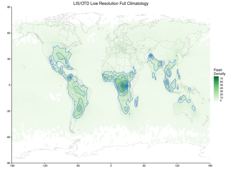
Low Resolution Full Climatology
The next step was to interrogate the contents of one of the HDF files. A given file may contain multiple data sets (this is part of the “hierarchical” nature of HDF), so we’ll check on what data sets are packed into one of those files. Let’s look at the Low Resolution Full Climatology (LRFC) data.
> file = h5file(name = "data/LISOTD\_LRFC\_V2.3.2014.h5", mode = "r")
> dataset = list.datasets(file)
> cat("datasets:", dataset, "\n")
datasets: /lrfc
Just a single data set, but that’s by design: we only extracted one using h5fromh4 above. What are the characteristics of that data set?
> print(file[dataset])
DataSet 'lrfc' (72 x 144)
type: numeric
chunksize: NA
maxdim: 72 x 144
It contains numerical data and has dimensions 72 by 144, which means that it has been projected onto a latitude/longitude grid with 2.5° resolution. We’ll just go ahead and read in those data.
> lrfc = readDataSet(file[dataset])
> class(lrfc)
[1] "matrix"
> dim(lrfc)
[1] 72 144
That wasn’t too hard. And it’s not much more complicated if there are multiple data sets per file.
Below is a plot showing the annualised distribution of lightning across the Earth’s surface. It’s apparent that most lightning occurs over land in the tropics, with the highest concentration in Central Africa. The units of the colour scale are flashes per square km per year. Higher resolution data can be found the HRFC file (High Resolution Full Climatology), but the LRFC is quite sufficient to get a flavour of the data.
Low Resolution Annual Climatology
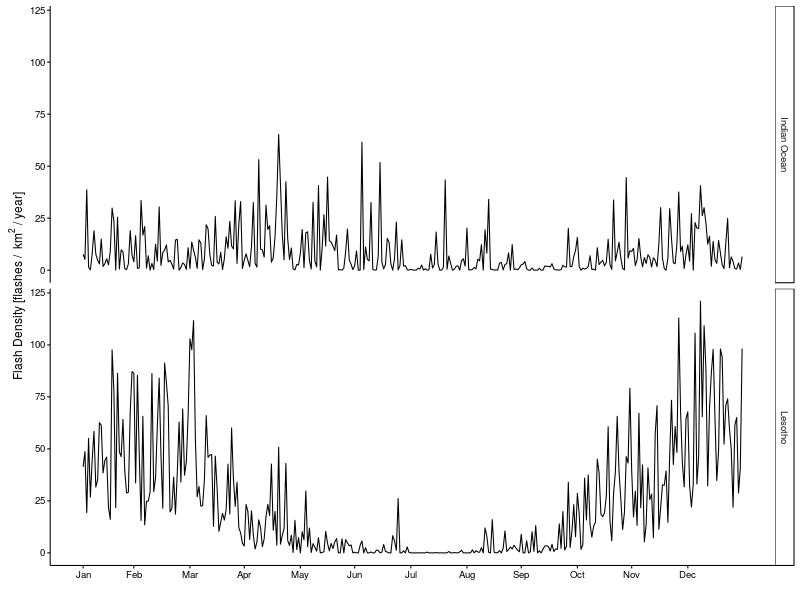
The Low Resolution Annual Climatology (LRAC) data have the same spatial resolution as LRFC but the data are broken down by day of year. This allows us to see how lightning activity varies at a particular location during the course of a year.
> file = h5file(name = "data/LISOTD\_LRFC\_V2.3.2014.h5", mode = "r")
> dataset = list.datasets(file)
> lrac = readDataSet(file[dataset])
> dim(lrac)
[1] 72 144 365
The data are now packed into a three dimensions array, where the first two dimensions are spatial (as for LRFC) and the third dimension corresponds to day of year.
We’ll look at two specific grid cells, one centred at 28.75° S 28.75° E (near the northern border of Lesotho, which according to the plot above is a region of relatively intense lightning activity) and the other at 31.25° S 31.25° E (in the Indian Ocean, just off the coast of Margate, South Africa). The annualised time series are plotted below. Lesotho has a clear annual cycle, with peak lightning activity during the Summer months but extending well into Spring and Autumn. There is very little lightning activity in Lesotho during Winter due to extremely dry and cold conditions. The cell over the Indian Ocean has a relatively high level of sustained lightning activity throughout the year. This is due to the presence of the warm Agulhas Current flowing down the east coast of South Africa. We wrote a paper about this, Processes driving thunderstorms over the Agulhas Current. It’s also open access, so go ahead and check it out.
Although the data in the plot above are rather jagged, with some aggregation and mild filtering they become pleasingly smooth and regular. We observed that you could actually fit the resulting curves rather well with just a pair of sinusoids. That work was documented in A harmonic model for the temporal variation of lightning activity over Africa. Like the other two papers, it’s open access. Enjoy (if that sort of thing is your cup of tea).
Conclusion
My original intention with this post was to show how to handle HDF data in R. But in retrospect it has achieved a second objective, showing that it’s possible to do some meaningful Science with data that’s in the public domain.