PLOS Subject Keywords: Gathering Data

I’m putting together a couple of articles on Collaborative Filtering and Association Rules. Naturally, the first step is finding suitable data for illustrative purposes.

There are a number of standard data sources for these kinds of analyses:

the MovieLens data (ratings of thousands of movies by millions of viewers);
the Jester data (ratings of jokes);
the Book-Crossing data (ratings of books);
the Last.fm data (music preferences);
the Amazon data (product reviews);
the Million Song Dataset Challenge on Kaggle;
the LibRec library has a collection of suitable data; and
a collection of data sets on Yahoo!.

I’d like to do something different though, so instead of using one of these, I’m going to build a data set based on subject keywords from articles published in PLOS journals. This has the advantage of presenting an additional data construction pipeline and the potential for revealing something new and interesting.

Before we get started, let’s establish some basic nomenclature.

Terms

Data used in the context of Collaborative Filtering or Association Rules analyses are normally thought of in the following terms:

Item: - a "thing" which is rated.
User: - a "person" who either rates one or more Items or consumes ratings for Items.
Rating: - the evaluation of an Item by a User (can be a binary, integer or real valued rating or simply whether or not the User has interacted with the Item).

Sample Article

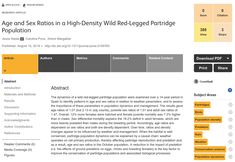
We’re going to retrieve a load of data from PLOS. But, just to set the scene, let’s start by looking at a specific article, Age and Sex Ratios in a High-Density Wild Red-Legged Partridge Population, recently published in PLOS ONE. You’ll notice that the article is in the public domain, so you can immediately download the PDF (no paywalls here!) and access a wide range of other data pertaining to the article. There’s a list of subject keywords on the right. This is where we will be focusing most of our attention, although we’ll also retrieve DOI, authors, publication date and journal information for good measure.

Article title and abstract from PLOS ONE.

We’ll be using the rplos package to access data via the PLOS API. A search through the PLOS catalog is initiated using searchplos(). To access the article above we’d just specify the appropriate DOI using the q (query) argument, while the fields in the result are determined by the fl argument.

library(rplos)
partridge <- searchplos(
  q = "id:10.1371/journal.pone.0159765",
  fl = 'id,author,publication_date,subject,journal'
)$data

The journal, publication date and author data are easy to consume.

partridge$id

[1] "10.1371/journal.pone.0159765"

partridge[, 3:5]

   journal     publication_date                                       author
1 PLOS ONE 2016-08-10T00:00:00Z Jesús Nadal; Carolina Ponz; Antoni Margalida

The subject keywords are conflated into a single string, making them more difficult to digest.

partridge$subject %>% cat

/Biology and life sciences/Population biology/Population dynamics;
/Ecology and environmental sciences/Conservation science;
/Earth sciences/Atmospheric science/Meteorology/Weather;
/Earth sciences/Atmospheric science/Meteorology/Rain;
/Ecology and environmental sciences/Ecology/Community ecology/Trophic interactions/Predation;
/Biology and life sciences/Ecology/Community ecology/Trophic interactions/Predation;
/Biology and life sciences/Population biology/Population metrics/Population density;
/Biology and life sciences/Organisms/Animals/Vertebrates/Amniotes/Birds;
/Biology and life sciences/Organisms/Animals/Vertebrates/Amniotes/Birds/Fowl/Gamefowl/Partridges

Here’s an extract from the documentation about subject keywords which helps make sense of that.

The Subject Area terms are related to each other with a system of broader/narrower term relationships. The thesaurus structure is a polyhierarchy, so for example the Subject Area "White blood cells" has two broader terms "Blood cells" and "Immune cells". At its deepest the hierarchy is ten tiers deep, with all terms tracking back to one or more of the top tier Subject Areas, such as "Biology and life sciences" or "Social sciences."

We’ll use the most specific terms in each of the subjects. It’d be handy to have a function to extract these systematically from a bunch of articles.

library(dplyr)
 
options(stringsAsFactors = FALSE)
split.subject <- function(subject) {
  data.frame(
    subject = sub(".*/", "", strsplit(subject, "; ")[[1]]),
    stringsAsFactors = FALSE
  ) %>%
  group_by(subject) %>%
  summarise(count = n()) %>%
  ungroup
}

So, for the article above we get the following subjects:

split.subject(partridge$subject)

# A tibble: 8 x 2
               subject count
                 <chr> <int>
1                Birds     1
2 Conservation science     1
3           Partridges     1
4   Population density     1
5  Population dynamics     1
6            Predation     2
7                 Rain     1
8              Weather     1

Those tie up well with what we saw on the home page for the article. We see that all of the terms except Predation appear only once. There are two entries for Predation, one in category “Ecology and environmental sciences” and the other in “Biology and life sciences”. We can’t really interpret these entries as ratings. They should rather be thought of as interactions. At some stage we might transform them into Boolean values, but for the moment we’ll leave them as interaction counts.

Some data is collected explicitly, perhaps by asking people to rate things, and some is collected casually, for example by watching what people buy. Toby Segaran, Programming Collective Intelligence

Article Collection

We’ll need a lot more data to do anything meaningful. So let’s use the same infrastructure to grab a few thousand articles.

dim(articles)

[1] 185984      5

Parsing the subject column and aggregating the results we get a data frame with counts of the number of times a particular subject keyword is associated with each article.

subjects <- lapply(1:nrow(articles), function(n) {
    cbind(
      doi = articles$id[n],
      journal = articles$journal[n],
      split.subject(articles$subject[n])
    )
  }) %>% bind_rows %>% mutate(
    subject = factor(subject)
  )
dim(subjects)

[1] 1433963       4

Here are the specific data for the article above:

subset(subjects, doi == "10.1371/journal.pone.0159765")

                                 doi  journal              subject count
1425105 10.1371/journal.pone.0159765 PLOS ONE                Birds     1
1425106 10.1371/journal.pone.0159765 PLOS ONE Conservation science     1
1425107 10.1371/journal.pone.0159765 PLOS ONE           Partridges     1
1425108 10.1371/journal.pone.0159765 PLOS ONE   Population density     1
1425109 10.1371/journal.pone.0159765 PLOS ONE  Population dynamics     1
1425110 10.1371/journal.pone.0159765 PLOS ONE            Predation     2
1425111 10.1371/journal.pone.0159765 PLOS ONE                 Rain     1
1425112 10.1371/journal.pone.0159765 PLOS ONE              Weather     1

Note that we’ve delayed the conversion of the subject column into a factor until all of the required levels were known.

In future instalments I’ll be looking at analyses of these data using Association Rules and Collaborative Filtering.