There are a variety of ways to predict running times over the standard marathon distance (42.2 km). You could dust off your copy of The Lore of Running (Tim Noakes). My treasured Third Edition discusses predicting likely marathon times on p. 366, referring to tables published by other authors to actually make predictions. There’s also a variety of online services, for example:
- Runners’ World’s Race Time Predictor (based on Riegel’s Formula),
- Running for Fitness’s Race Predictor and
- Race Result Predictor.
Of these I particularly like the offering from Running for Fitness which produces a neatly tabulated set of predicted times over an extensive range of distances using a selection of techniques including Riegel’s Formula and Cameron’s Model.
While the sites listed above certainly provide useful predictions, I have a niggling feeling that they aren’t fully exploiting the large amount of data that we currently have available (both as individual athletes and as a global fraternity of runners). I’ve developed a relentless itch to provide a better solution. I wanted to do the following:
- incorporate information for multiple measurements (other solutions just use a single time over another distance);
- illustrate how the prediction is updated (and hopefully improved) by adding additional measurements;
- provide an indication of uncertainty in the prediction.
Using data accumulated from a number of races in South Africa I put together a Bayesian model for prediction marathon times. The likelihood function, which embodies the code data for the model, was constructed using npcdensbw() and npcdens() from the np package (nonparametric kernel smoothing methods for mixed data types).
| Distance [km] | Time [HH:MM] | Marathon (Riegel's Formula) [HH:MM] |
|---|---|---|
| 10.0 | 00:38 | 02:55 |
| 21.1 | 01:17 | 02:40 |
| 25.0 | 01:34 | 02:43 |
| 32.0 | 01:59 | 02:40 |
The third column is the predicted marathon time using Riegel’s Formula on the time achieved over each distance.
Actual marathon time for this runner is 2:42.
But the mode of the posterior is at 170 minutes.
We start with a belief, called a prior. Then we obtain some data and use it to update our belief. The outcome is called a posterior. Should we obtain even more data, the old posterior becomes a new prior and the cycle repeats.
Below is the default prior distribution constructed as the distribution of all marathon times in the data set. In the absence of further information regarding a particular runner, this is a reasonable guess for the distribution of possible marathon times. It represents our initial belief of what’s possible.
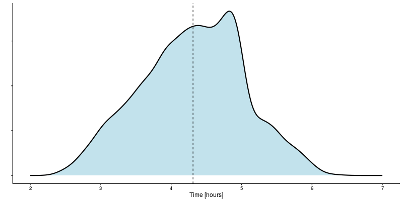
Based on the default prior the expected time for finishing a marathon is 04:19, with a 95% confidence interval that extends from 02:51 to 05:43.
Once we have some data though, we are able to update the initial belief using Bayes’ Theorem to generate a posterior distribution.
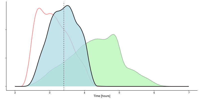
Having incorporated the 10 km finishing time, the expected marathon time drops to 03:24. Quite an improvement! The 95% confidence interval also narrows to between 02:38 and 04:07.
When further information becomes available, the current posterior distribution becomes the prior for the next application of Bayes’ Theorem. This cycle repeats itself with each new piece of information, the posterior progressively becoming a more accurate representation of the information captured in the measurements.
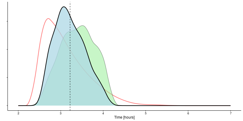
Adding a time of 01:17 over 21.1 km into the mix gives an expected marathon time of 03:13, slicing off another 11 minutes.
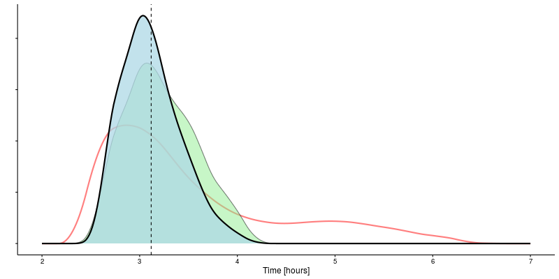
A time of 01:34 for 25 km gives the expected marathon time another boost to 03:07.
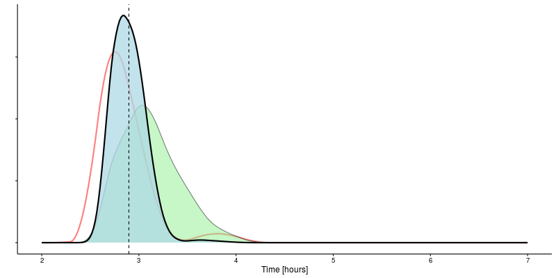
Finally, adding in a time of 01:59 for 32 km drops the anticipated marathon time down to 02:54, with a 95% confidence interval from 02:36 to 03:16.