Clustering Time Series Data

I have been looking at methods for clustering time domain data and recently read TSclust: An R Package for Time Series Clustering by Pablo Montero and José Vilar. Here are the results of my initial experiments with the TSclust package.

Grabbing Some Data

Since stock ticker data are not too dissimilar to the data that I am currently working with, they seemed like a reasonable target for my experiments.

library(quantmod)
symbols = c('A', 'AAPL', 'ADBE', 'AMD', 'AMZN', 'BA', 'CL', 'CSCO',
            'EXPE', 'FB', 'GOOGL', 'GRMN', 'IBM', 'INTC', 'LMT', 'MSFT',
            'NFLX', 'ORCL', 'RHT', 'YHOO')

start = as.Date("2014-01-01")
until = as.Date("2014-12-31")

# Grab data, selecting only the Adjusted close price.
#
stocks = lapply(symbols, function(symbol) {
   adjusted = getSymbols(
      symbol,
      from = start,
      to = until,
      auto.assign = FALSE
   )[, 6]
   names(adjusted) = symbol
   adjusted
})

# Merge by date
#
stocks = do.call(merge.xts, stocks)

# Convert from xts object to a matrix (since xts not supported as input
# for TSclust). Also need to transpose because diss() expects data to be
# along rows.
#
stocks = t(as.matrix(stocks))

Just to get an idea of what these data look like, we can put together a compound time series plot.

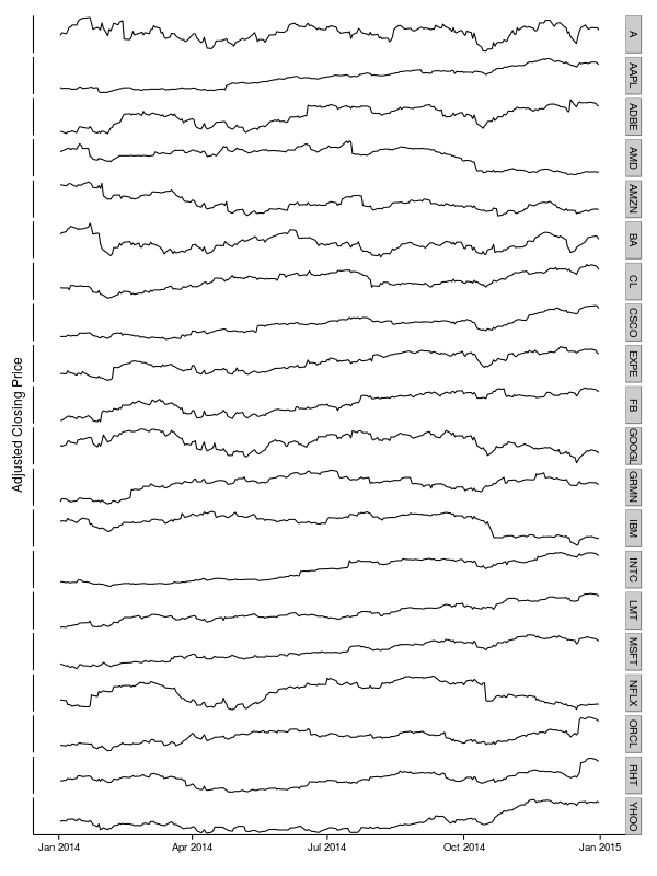
Time series of adjusted closing price for a selection of stocks.

No great similarities jump out at the naked eye, so let’s see what a bit of Machine Learning has to offer.

Clustering in the Time Domain

The TSclust package offers a range of algorithms for calculating the dissimilarity measure between time series. The diss() function serves as a wrapper for accessing the various algorithms. The package caters for more than 20 algorithms and we’ll just take a look at a representative sample here.

Correlation

Correlation is an obvious option when considering the degree of similarity between time series. Generating a dissimilarity matrix is simple.

D1 <- diss(stocks, "COR")
summary(D1)

   Min. 1st Qu.  Median    Mean 3rd Qu.    Max. 
 0.3275  0.8860  1.2350  1.1890  1.5180  1.8940

Note that, since this is a measure of dissimilarity, the range of correlation has been shifted from [-1,1] to [0,2]. To get an idea of what the dissimilarity data look like, we’ll look at a mosaic plot. There appear to be blocks of similar stocks. For example, INTC, LMT and MSFT are not too dissimilar to each other. They are also not dissimilar to CSCO, EXPE or FB. But they are very different to AMD and AMZN.

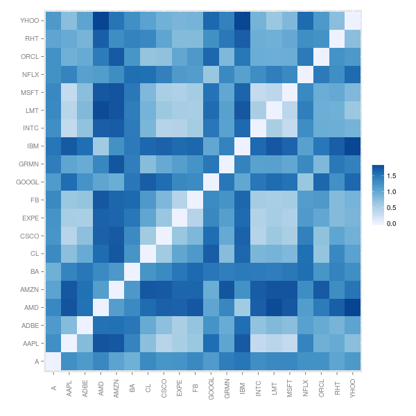
Heat map showing a dissimilarity matrix for pairs of stocks based on correlation.

Which stocks present the most unique time series? It looks like AMZN, IBM and AMD differ consistently from most of the other stocks considered.

sort(rowMeans(as.matrix(D1)))

     EXPE      INTC      AAPL      MSFT      CSCO      ADBE       LMT 
0.9378181 0.9394791 0.9456821 0.9502528 0.9625090 0.9820178 0.9837705 
       FB        CL       RHT      ORCL      YHOO      GRMN         A 
1.0058017 1.0941648 1.0961343 1.0967862 1.1144521 1.1701074 1.1894821 
     NFLX     GOOGL        BA       AMD       IBM      AMZN 
1.2336638 1.2969912 1.3212228 1.4211540 1.4238809 1.4330921

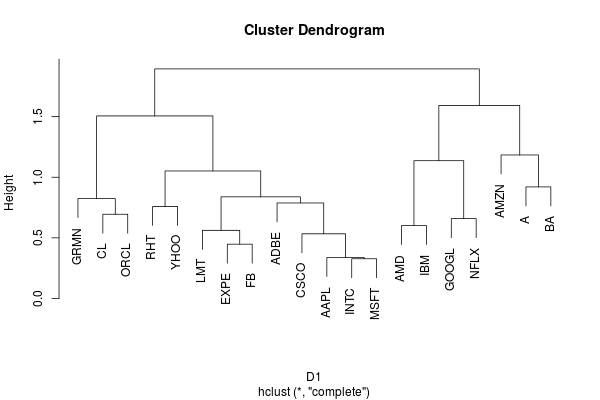
Now let’s use those data to do some hierarchical clustering.

C1 <- hclust(D1)

Looking at the dendrogram below, it appears that a cut at a height of around 1.25 would divide the stocks into four groups. Not too surprisingly, INTC, LMT and MSFT end up in the same group along with CSCO, EXPE and FB.

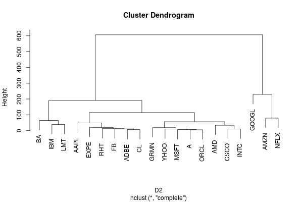
A hierarchical clustering tree for stocks based on time series data using correlation distance.

Fréchet Distance

Next we’ll try out the Fréchet Distance, which is a somewhat esoteric measure of the difference between two curves (or two time series) and has been applied to problems like recognition of handwritten documents and protein structure alignment.

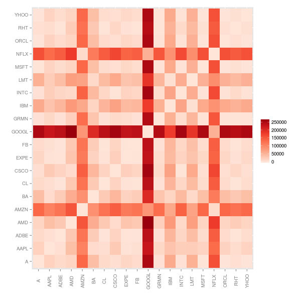
D2 <- diss(stocks, "FRECHET")

The resulting dissimilarity matrix is profoundly different, with AMZN, GOOGL and NFLX standing out as significantly different to the other time series.

Heat map showing a dissimilarity matrix for pairs of stocks based on Fréchet distance.

This results in a tree structure with essentially two branches: AMZN, GOOGL and NFLX on one branch and the rest of the stocks on the other branch. Within the second branch LMT, IBM and BA are also clustered together.

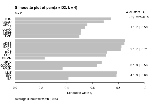
A hierarchical clustering tree for stocks based on time series data using Fréchet distance.

Dynamic Time Warping Distance

Dynamic Time Warping is a technique for comparing time series where the timing or the tempo of the variations may vary between the series.

D3 <- diss(stocks, "DTWARP")

The Dynamic Time Warping dissimilarity matrix is reminiscent of the one we got from the Fréchet Distance, with AMZN, GOOGL and NFLX clearly differentiated.

Heat map showing a dissimilarity matrix for pairs of stocks based on Dynamic Time Warping distance.

Since the dissimilarity matrix is similar to one we’ve already looked at, we’ll try a different approach to clustering, using the Partitioning Around Medoids (PAM) algorithm. Looking at the associated silhouette plot we can see that the high level structure is similar: AMZN, GOOGL and NFLX are clustered in one branch, while LMT, IBM and BA are in another.

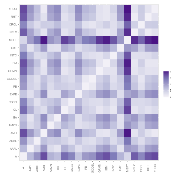
A silhouette plot for a PAM tree based on stocks time series data using Dynamic Time Warping distance.

Integrated Periodogram Distance

The integrated Periodogram is a variation of the periodogram where the power is accumulated as a function of frequency. This is a more robust measure for the purposes of comparing spectra. Signals with comparable integrated periodograms will contain variations at similar frequencies.

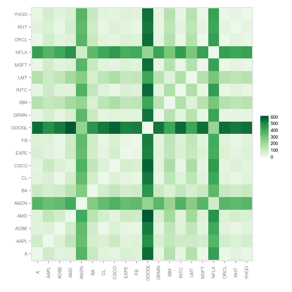
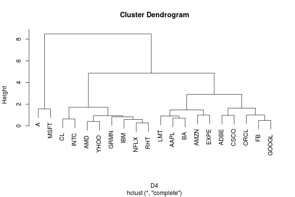
D4 <- diss(stocks, "INT.PER")

The dissimilarity matrix paints yet another picture of the data. In this view MSFT stands out as being significantly different from most of the other stocks.

Heat map showing a dissimilarity matrix for pairs of stocks based on Integrated Periodogram distance.

A hierarchical clustering tree for stocks based on time series data using Integrated Periodogram distance.

Conclusion

A different view of these data would obviously have been obtained if we had clustered the returns rather than the closing prices themselves.