Old 'Hood, New 'Hood

I recently moved from suburban South Africa to rural England. I’m figuring out my new environment. Making some maps seemed to be a good way to get familiar with the surroundings.

In the process I wanted to figure out two things:

• how to get maps with a consistent aspect ratio at different latitudes; and
• how to overlay a partially transparent map layer.

To make things more interesting I’ll create maps of both my old and new locations.

Let’s pull in a few libraries.

library(geosphere)
library(ggmap)

Distance and Latitude

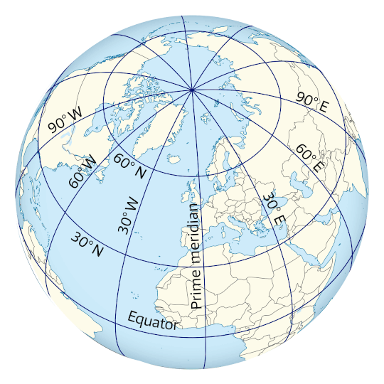
Let’s figure out the aspect ratio issue first. This arises because lines of longitude converge at the poles. As a result, a map with the same latitudinal and longitudinal extent, say 1° by 1°, looks very different at 60° latitude than it does at the equator.

We can illustrate this by estimating the distances using the Haversine formula (which assumes a spherical Earth).

# 1° of longitude on the Equator.
distHaversine(c(0, 0), c(1, 0))

[1] 111319.5

# 1° of longitude at 60° latitude.
distHaversine(c(0, 60), c(1, 60))

[1] 55659.22

Twice as long at the equator! A plot illustrates this effect rather nicely.

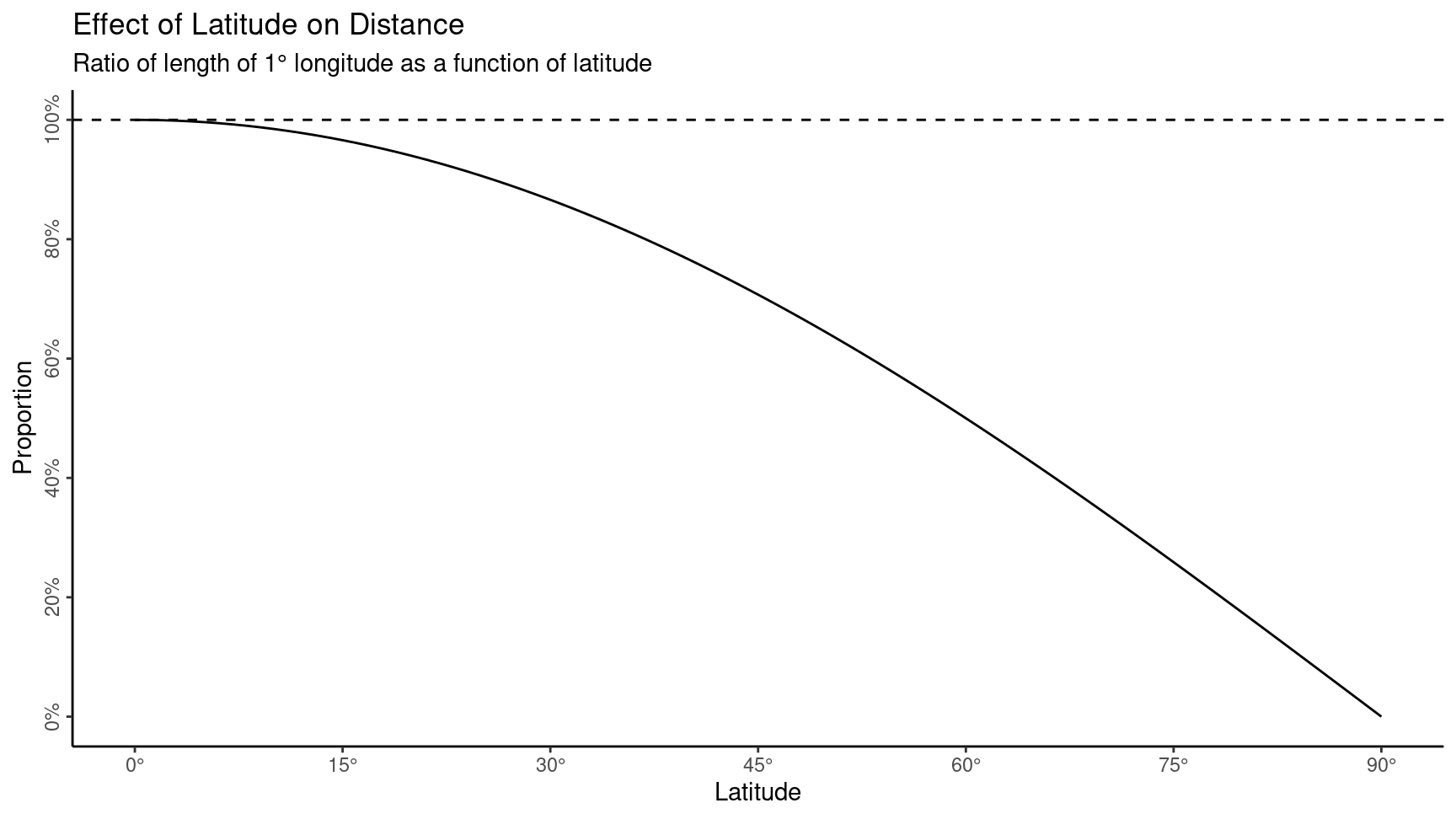
Why is this important? Well, it means that 1° by 1° maps at the equator and at 60° latitude will represent very different areas and have different aspect ratios. 💡 For presentation purposes, this effect can be mitigated by choosing an appropriate map projection.

Mercator & Pseudo-Mercator

The Pseudo-Mercator (or Web Mercator) projection is a variation on the Mercator projection which is commonly used for maps on the internet. The maps served by Google Maps and OpenStreetMap, for example, use the Pseudo-Mercator projection. The Pseudo-Mercator projection treats the Earth as a sphere, while the Mercator projection takes into account the fact that the Earth is actually an oblate, ellipsoidal or “squashed” sphere. It’s not very squashed, but it’s squashed enough to make a difference.

Both projections produce maps which look familiar: lines of latitude and longitude are straight, North is at the top, area gets bigger at higher latitudes. The differences are fairly subtle and really only relate to how angles on the surface of the Earth differ from angles on the map. For many applications this is not terribly important.

Why is the Pseudo-Mercator projection used for maps on the internet? It seems that this is ostensibly due to the different computational requirements: the maths for a spherical Earth is simpler (and quicker) than the maths for an ellipsoidal Earth.

Aspect Ratio

I wanted a simple way to calculate the aspect ratio of a 1° by 1° piece of the Earth’s surface as a function of latitude.

map_aspect <- function(lat, delta = 0.5) {
  if (lat + delta > 90) {
    NA
  } else {
    lon <- distHaversine(c(-delta, lat), c(delta, lat))
    lat <- distHaversine(c(0, lat - delta), c(0, lat + delta))
    lat / lon
  }
}

How does that vary with latitude?

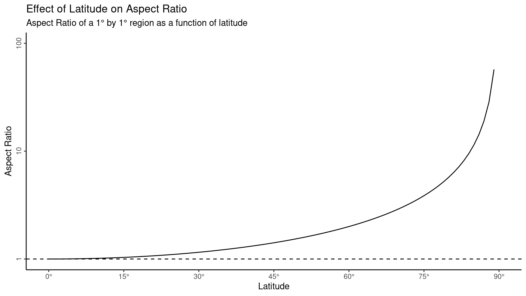
The scale on the vertical axis is logarithmic. The aspect ratio does really get large closer to the poles, where the 1° by 1° region is very narrow indeed.

How am I planning on using this? I want to plot maps for two regions at different latitudes. But I also want the maps to have the same aspect ratio. I need to specify a latitude-longitude bounding box for each map. I start by choosing the height I want the map to be (difference in latitude between top and bottom edges), then I use the aspect ratio to calculate the appropriate width (difference in longitude between left and right edges). Let’s give it a try.

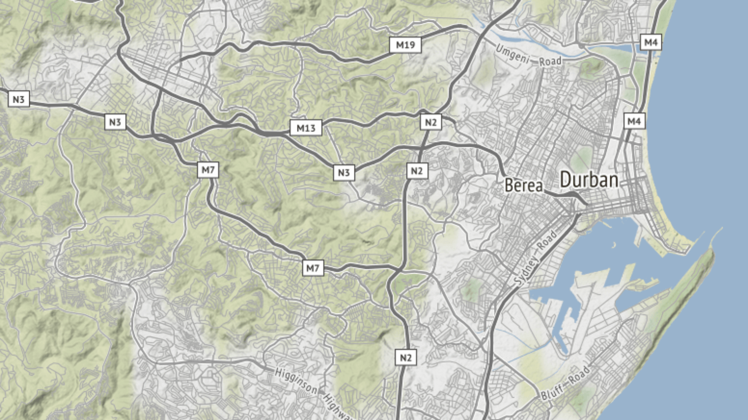
First a map of Durban, South Africa.

Then a map of West Berkshire, England.

Both of these maps use the terrain-background tiles from Stamen Design.

That feels a little underwhelming? Was all this messing around with aspect ratios worth it? I think it was. I now have two maps with the same shape and which represent the same distance along the vertical axis. And that’s pretty cool. To me, anyway.

Transparent Map Layers

I wanted to be able to stack multiple map layers with varying levels of transparency. Although ggmap() has a darken argument, this doesn’t do the job. I did some research and did not find a good solution. So I rolled my own.

#' Add transparency to a ggmap object
#'
#' Add an alpha (transparency) layer to a \code{ggmap} object. This makes it
#' possible to superimpose multiple map layers and have the lower layers shine
#' through.
#'
#' @param map A \code{ggmap} object.
#' @param alpha The required transparency (a number between 0 and 1).
#'
#' @return A \code{ggmap} object.
#' @export
#'
#' @examples
#' zoom <- 12
#' bbox <- c(-0.3275, 51.407222, 0.0725, 51.607222)
#'
#' base <- get_map(bbox, zoom, maptype = "terrain-lines")
#' overlay <- get_map(bbox, zoom, maptype = "watercolor")
#'
#' # Plot the base map.
#' ggmap(base)
#' # Plot the overlay map (100% opacity).
#' ggmap(overlay)
#'
#' # Plot the base map with the overlay superimposed at 25% opacity.
#' ggmap(base) +
#'   inset_ggmap(
#'     set_map_alpha(overlay, 0.25)
#'   )
set_map_alpha <- function(map, alpha) {
  if(class(map)[1] != "ggmap") {
    stop("map must be a ggmap object", call. = FALSE)
  }
  if(class(alpha) != "numeric" || alpha < 0 || alpha > 1) {
    stop("alpha must be a number between 0 and 1", call. = FALSE)
  }
  
  # Record the attributes & dimensions of the map object.
  map_attributes <- attributes(map)
  map_dimensions <- dim(map)
  
  # Add an alpha channel.
  map <- grDevices::adjustcolor(map, alpha)
  
  # Add back the dimensions (convert vector to matrix).
  dim(map) <- map_dimensions
  # Add back the attributes.
  attributes(map) <- map_attributes
  
  # Convert from matrix to map.
  class(map) <- c("ggmap", "raster")
  
  map
}

The set_map_alpha() function above accepts a map (returned by get_map()) and an alpha (between 0 and 1), then creates an alpha channel on the map.

The approach is nothing magical:

1. accept a ggmap object;
2. record the attributes and (pixel) dimensions;
3. use the builtin adjustcolor() function to add an alpha layer (the underlying data structure of the map is essentially a matrix of RGB strings);
4. the previous step results in a vector, so add back the dimensions, turning it into a matrix;
5. add back the attributes; and
6. convert to a ggmap object by assigning to class().

The Maps

Let’s try this out on those maps. I’ve created two versions of the Durban map, durban_terrain_lines and durban_terrain_background, which use the terrain-lines and terrain-background tiles from Stamen Design. For the latter I’ve used set_map_alpha() to add an alpha channel. To create an overlaid map I use ggmap() to create the base layer and then superimpose another later using inset_ggmap().

ggmap(durban_terrain_lines) +
  inset_ggmap(durban_terrain_background)

How does that look? This is the Durban map with a terrain-lines base and a terrain-background overlay at 50% opacity.

And now the West Berkshire map with a terrain-lines base and a watercolor overlay at 30% opacity.

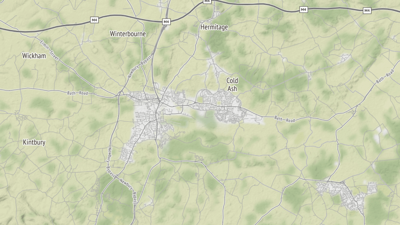
I really like the detail one can see on the terrain-lines map with a hint of colour from the overlaying, transparent layers.

It’s apparent that my new environment is substantially different to where I was before. My old ‘hood was great, but my new ‘hood is better.

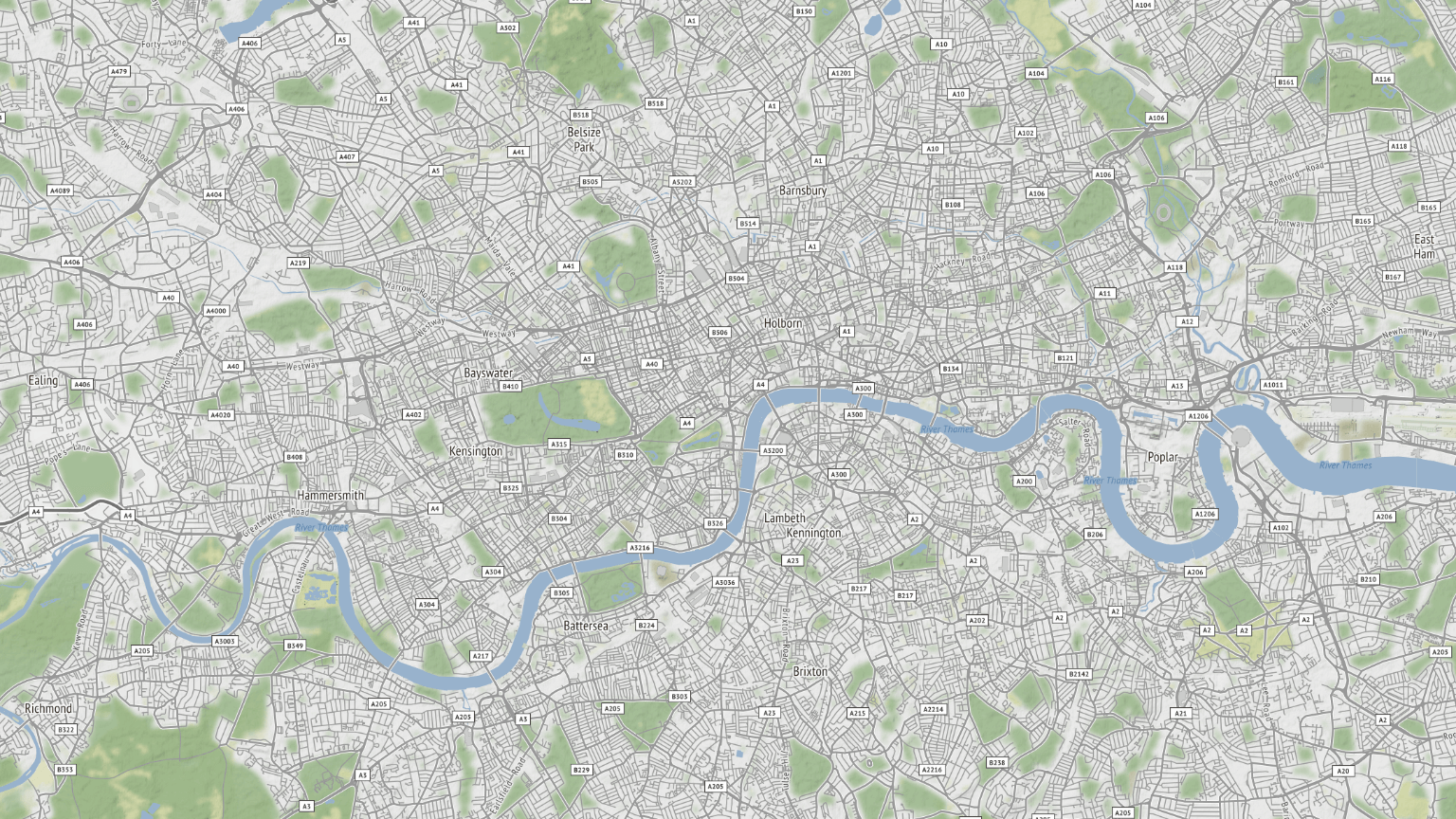
Epilogue

Finally, just going to throw this in here because I think it looks cool: a map of London with multiple layers.

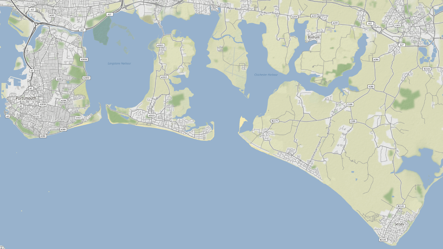
Also, just because I’m having fun, here’s a map from an area where we took a short vacation in Hampshire and West Sussex.