The key to successful backtesting is to ensure that you only use the data that were available at the time of the prediction. No “future” data can be included in the model training set, otherwise the model will suffer from look-ahead bias (having unrealistic access to future data).
One way to avoid look-ahead bias is to iterate over the data, repeatedly fitting and forecasting, while ensuring that the model is only ever fit to historical data. This can be laborious and error-prone. With the {rugarch} package a better option is to use the ugarchroll() function which will “roll” along the data, fitting and predicting as it goes.
Moving Window
A moving (or rolling) window of fixed length moves along the data, fitting and testing the model as it goes. You need not refit the model at each time step.
specification <- ugarchspec(
  mean.model = list(armaOrder = c(0, 0)),
  variance.model = list(model = "sGARCH"),
  distribution.model = "sstd"
)

rolling <- ugarchroll(
  specification,
  data = TATASTEEL,
  n.start = 500,
  refit.every = 50,
  refit.window = "moving"
)
The new parameters required to get this working are: n.start, refit.window and refit.every. What do these parameters mean?
n.start— number of time steps in window;refit.window— type of window ("moving","recursive"or"expanding");refit.every— number of time steps between refitting the model.
The refit frequency should be determined by how dynamic your data is. If the nature of the data often changes then you’ll want to refit more frequently (smaller refit.every).
Let’s take a look at the results of the rolling fit.
rolling
*-------------------------------------*
*              GARCH Roll             *
*-------------------------------------*
No.Refits       : 20
Refit Horizon   : 50
No.Forecasts    : 984
GARCH Model     : sGARCH(1,1)
Distribution    : sstd

Forecast Density:
               Mu  Sigma   Skew  Shape Shape(GIG) Realized
2018-01-10 0.0023 0.0138 1.1313 4.9882          0   0.0042
2018-01-11 0.0023 0.0137 1.1313 4.9882          0  -0.0062
2018-01-12 0.0023 0.0136 1.1313 4.9882          0  -0.0012
2018-01-15 0.0023 0.0136 1.1313 4.9882          0   0.0150
2018-01-16 0.0023 0.0135 1.1313 4.9882          0  -0.0165
2018-01-17 0.0023 0.0136 1.1313 4.9882          0   0.0108

..........................
               Mu  Sigma   Skew  Shape Shape(GIG) Realized
2021-12-24 0.0035 0.0268 1.0265 5.0374          0  -0.0084
2021-12-27 0.0035 0.0263 1.0265 5.0374          0   0.0067
2021-12-28 0.0035 0.0257 1.0265 5.0374          0   0.0022
2021-12-29 0.0035 0.0251 1.0265 5.0374          0  -0.0100
2021-12-30 0.0035 0.0248 1.0265 5.0374          0  -0.0125
2021-12-31 0.0035 0.0246 1.0265 5.0374          0   0.0095

Elapsed: 2.941511 secs
Where does the number of refits come from? It’s determined by the parameters listed above. We can check:
(nrow(TATASTEEL) - 500) %/% 50[1] 19And, of course, you need to add 1 to that for the initial fit.
Plots
The resulting object has a specialised plot() method that allows you to access various views via the which parameter. Let’s start by comparing the predicted and realised returns.
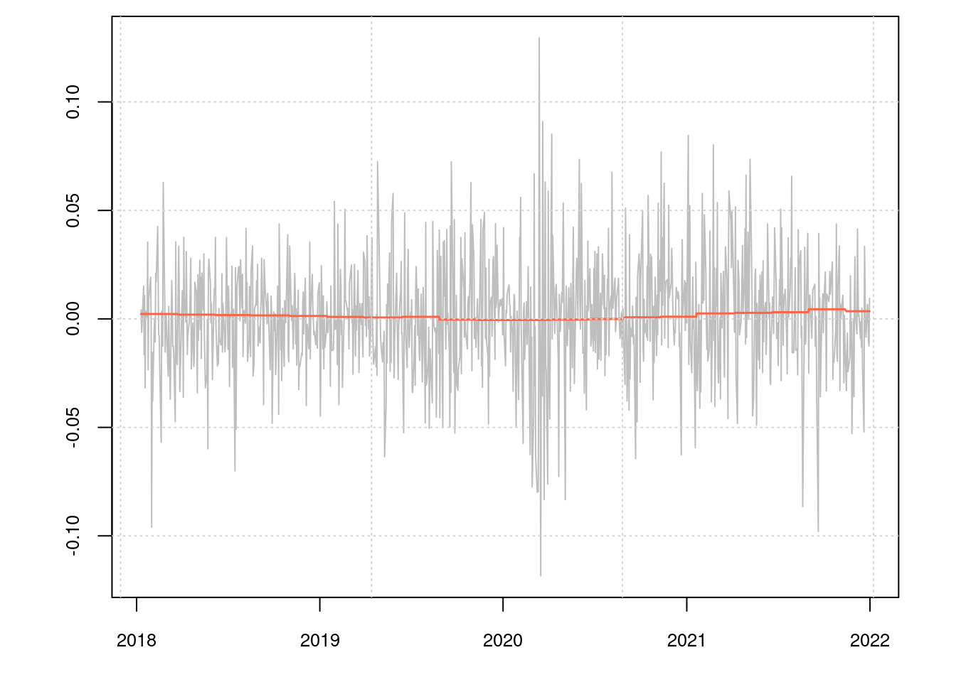
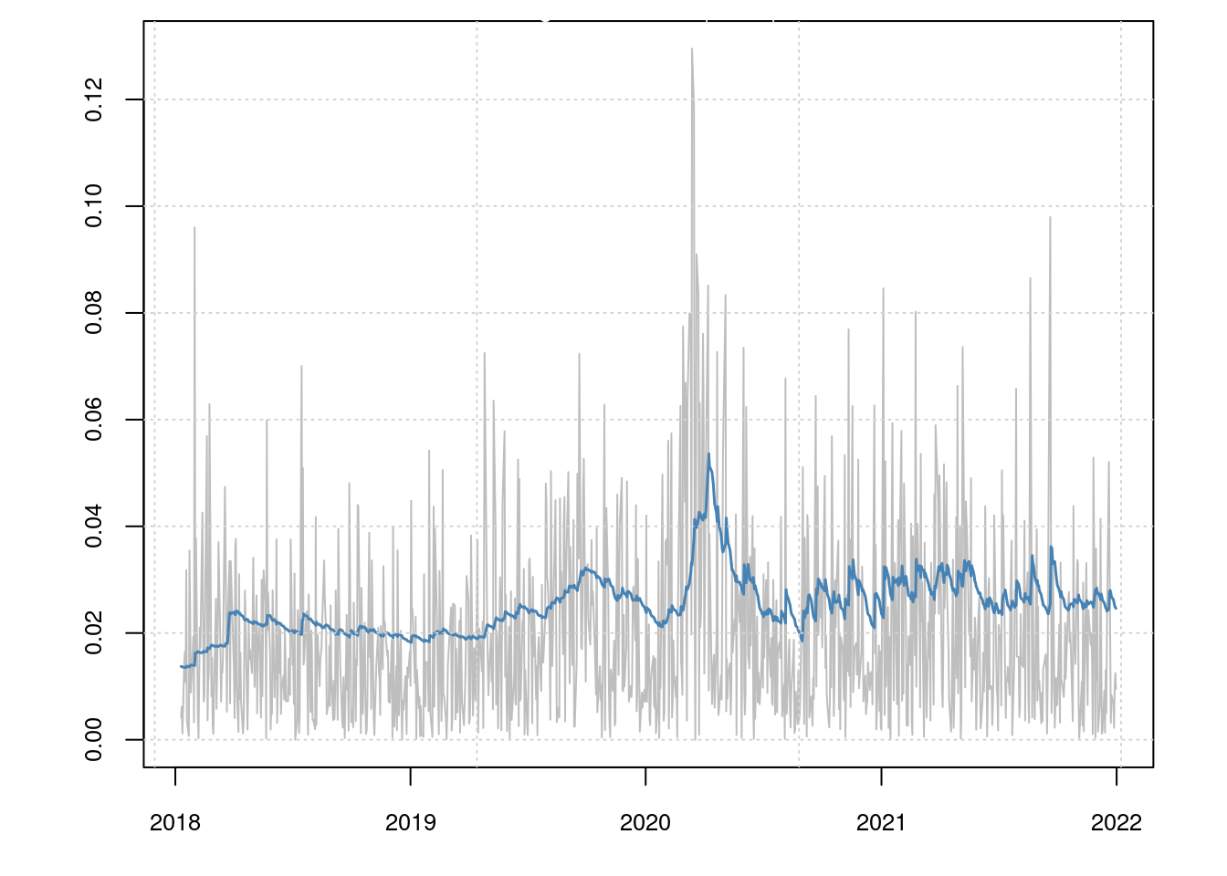
The agreement is not terribly good. However, for a GARCH model the focus is more on modelling the volatility than the returns themselves. Let’s compare the predicted and realised volatilities.
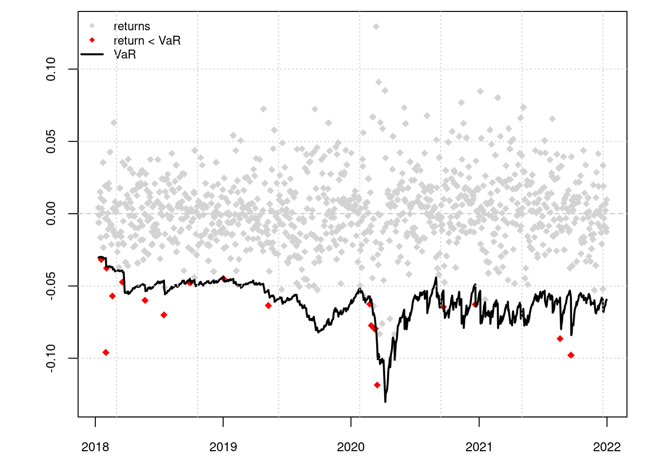
A Value at Risk (VaR) plot shows how the estimated risk associated with this asset changes over time. Exceedances (indicated by red diamonds) indicate days when the actual (negative) return is worse than that predicted by the model.
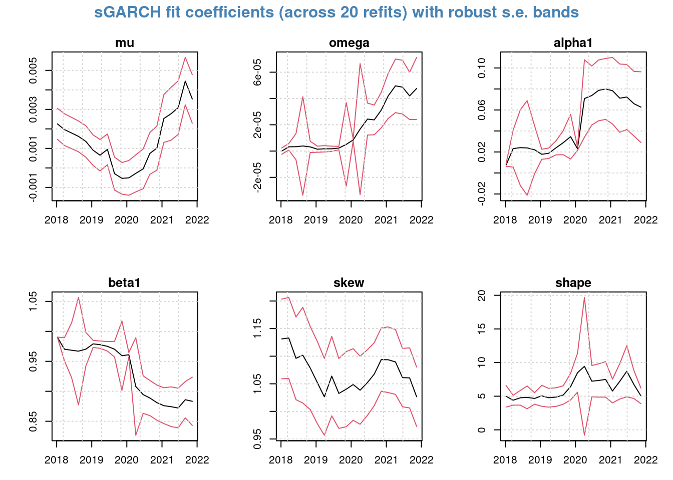
Finally, since we are refitting the model periodically the model coefficients also change with time.
Reports
Now let’s generate a VaR report using the backtest data.
report(rolling, type="VaR", VaR.alpha = 0.01, conf.level = 0.95)VaR Backtest Report
===========================================
Model: sGARCH-sstd
Backtest Length: 984
Data:
==========================================
alpha: 1%
Expected Exceed: 9.8
Actual VaR Exceed: 19
Actual %: 1.9%
Unconditional Coverage (Kupiec)
Null-Hypothesis: Correct Exceedances
LR.uc Statistic: 6.77
LR.uc Critical: 3.841
LR.uc p-value: 0.009
Reject Null: YES
Conditional Coverage (Christoffersen)
Null-Hypothesis: Correct Exceedances and
Independence of Failures
LR.cc Statistic: 7.552
LR.cc Critical: 5.991
LR.cc p-value: 0.023
Reject Null: YESThe VaR.alpha parameter is the tail probability and the conf.level parameter specifies the confidence level for the conditional coverage test.
The report presents results for two tests:
- Kupiec Test — Checks whether the number of exceedances is consistent with the confidence level of the VaR model.
- Christoffersen Test — Checks whether the number of exceedances is consistent with the confidence level of the VaR model and if the exceedances are independent.
The report indicates that both of these tests fail at the specified levels (both reject the null hypothesis).
The Forecast Performance Measures report gives another view on the backtest, providing some metrics on the models’ ability to predict the returns. It generates the following statistics:
MSE— Mean Square Error;MAE— Mean Absolute Error; andDAC— Directional Accuracy.
report(rolling, type="fpm")
GARCH Roll Mean Forecast Performance Measures
---------------------------------------------
Model       : sGARCH
No.Refits   : 20
No.Forecasts: 984

        Stats
MSE 0.0006922
MAE 0.0194600
DAC 0.4878000
Where do those metrics come from? Here’s how you can calculate the MSE manually:
predictions <- as.data.frame(rolling)

error <- predictions$Realized - predictions$Mu
mean(error^2)
[1] 0.000692193Model Coefficients
Since we built multiple models the coefficients are returned in a list, with an element in the list corresponding to each model.
coefficients <- coef(rolling)How many models were built?
length(coefficients)[1] 20The coefficients for the first model:
first(coefficients)$index
[1] "2018-01-09"
$coef
Estimate Std. Error t value Pr(>|t|)
mu 2.257802e-03 7.946035e-04 2.841420e+00 4.491311e-03
omega 8.634389e-12 2.413674e-06 3.577280e-06 9.999971e-01
alpha1 7.568079e-03 1.261387e-03 5.999807e+00 1.975516e-09
beta1 9.900565e-01 2.522851e-04 3.924356e+03 0.000000e+00
skew 1.131276e+00 7.219237e-02 1.567030e+01 0.000000e+00
shape 4.988236e+00 1.609348e+00 3.099538e+00 1.938230e-03The coefficients for the last model:
last(coefficients)$index
[1] "2021-11-12"
$coef
Estimate Std. Error t value Pr(>|t|)
mu 3.535174e-03 1.242213e-03 2.845868 4.429055e-03
omega 4.763787e-05 2.357402e-05 2.020778 4.330271e-02
alpha1 6.264364e-02 3.369790e-02 1.858978 6.303028e-02
beta1 8.833370e-01 4.022516e-02 21.959812 0.000000e+00
skew 1.026491e+00 5.380944e-02 19.076415 0.000000e+00
shape 5.037409e+00 1.156960e+00 4.354006 1.336721e-05Being able to interrogate each of the individual models is useful because we can see if there are insignificant model coefficients. These data are complimentary to the model coefficient plots above.
Comparing Models
Now we’ll repeat the process for another model, replacing "sstd" with "std" and using AR(1) rather than constant mean.
specification <- ugarchspec(
  mean.model = list(armaOrder = c(1, 0), include.mean = TRUE),
  variance.model = list(model = "sGARCH"),
  distribution.model = "std"
)

rolling <- ugarchroll(
  specification,
  data = TATASTEEL,
  n.start = 500,
  refit.every = 50,
  refit.window = "moving"
)
What is the Value at Risk performance?
report(rolling, type="VaR", VaR.alpha = 0.01, conf.level = 0.95)VaR Backtest Report
===========================================
Model: sGARCH-std
Backtest Length: 984
Data:
==========================================
alpha: 1%
Expected Exceed: 9.8
Actual VaR Exceed: 15
Actual %: 1.5%
Unconditional Coverage (Kupiec)
Null-Hypothesis: Correct Exceedances
LR.uc Statistic: 2.355
LR.uc Critical: 3.841
LR.uc p-value: 0.125
Reject Null: NO
Conditional Coverage (Christoffersen)
Null-Hypothesis: Correct Exceedances and
Independence of Failures
LR.cc Statistic: 3.845
LR.cc Critical: 5.991
LR.cc p-value: 0.146
Reject Null: NOLooks a bit better! Fewer exceedances and both tests are now passing, meaning that the null hypotheses (exceedances consistent with the specified confidence level) should not be rejected.
Expanding Window
An expanding or recursive window includes _all_previous data.
A moving window is generally a good option because the model is being retrained on the same volume of data each time. However, perhaps you want to train each model on all previous data? In this case use an "expanding" refit window.
rolling <- ugarchroll(
  specification,
  data = TATASTEEL,
  n.start = 500,
  refit.window = "expanding",
  refit.every = 50
)
Alternative Implementation
You can also do backtesting with the {tsgarch} package.
specification <- garch_modelspec(
  TATASTEEL,
  model = "gjrgarch",
  distribution = "sstd",
  constant = FALSE,
  order = c(1, 0)
)
backtest <- tsbacktest(
specification,
start = 500,
h = 1,
estimate_every = 50,
rolling = TRUE
)At present there do not appear to be utilities comparable to those in {rugarch} for analysing the results of the backtest and this currently needs to be done by hand.