In general a parsimonious model is a good model. A model with too many parameters is likely to overfit the data. How do we determine when a model is “complex enough” but not “too complex”?
We can use a significance test to determine whether the value of each parameter is significantly different from its null value. For many parameters the null value will simply be 0 but, as we will see, there are some parameters for which this is not true.
Parameter Significance
Parameter estimates will invariably be non-zero. This is because those estimates are obtained using numerical techniques. And those techniques might converge on a value of 0.001 or 0.000000857 (or any other really tiny value) for a parameter where the true value is precisely zero.
We can use a statistical test to determine whether the estimated value is significantly different from zero (“significant” in the sense that it is still different from zero taking into account the uncertainty associated with the numerical method).
AR(1) Model
Let’s start by building a GJR GARCH model for the Tata Steel returns, using a Skewed Student-t Distribution and modelling the mean as an AR(1) process.
flexible <- ugarchspec(
  mean.model = list(armaOrder = c(1, 0)),
  variance.model = list(model = "gjrGARCH"),
  distribution.model = "sstd"
)

overfit <- ugarchfit(data = TATASTEEL, spec = flexible)
This model has eight parameters. Is that too many?
coef(overfit) mu ar1 omega alpha1 beta1 gamma1 skew shape
1.308881e-03 -3.061775e-02 7.479402e-06 1.052012e-02 9.516515e-01 5.658366e-02 1.050847e+00 5.051158e+00 Looking at the parameter estimates alone is not enough to make a decision on the validity of the parameter estimates. A few of the estimates are pretty close to zero. But are they close enough that they are effectively zero? We need more information to make a decision on this point. Specifically, we need to know what the associated uncertainties are because these will provide us with a suitable scale to evaluate “close enough”.
We have to make a relatively obscure incantation to get the information that we need, looking at the matcoef element on the fit slot of the model object. This gives us the parameter estimates, the standard errors, t-statistics and \(p\)-values.
round(overfit@fit$matcoef, 3) Estimate Std. Error t value Pr(>|t|)
mu 0.001 0.001 2.316 0.021
ar1 -0.031 0.024 -1.257 0.209
omega 0.000 0.000 2.560 0.010
alpha1 0.011 0.003 3.125 0.002
beta1 0.952 0.006 147.897 0.000
gamma1 0.057 0.016 3.569 0.000
skew 1.051 0.037 28.516 0.000
shape 5.051 0.658 7.674 0.000The t-statistic is the ratio of the parameter estimate to the standard error. Larger (absolute) values are more significant. A rule of thumb for assessing the t-statistic:
If the t-statistic is greater than 2 then reject the null hypothesis at the 5% level.
This means that if the parameter estimate differs from the null value by more than two standard errors then it is regarded as significant.
The default null hypothesis is that the parameter is zero (that is, the null value is zero). Most of the parameter estimates are significant. For example, the value for shape seems to be obviously non-zero, and if we consider the associated standard error then we see that it differs from zero by a few standard errors. It’s a safe bet. The value for alpha1 is rather small and one might be tempted to think that it’s effectively zero. However, if you take into account the associated standard error then you see that it’s actually a few standard errors away from zero. It’s also safely significant.
Things are different with the estimate for ar1 though. The value is just a little more than one standard error away from zero and so is not statistically significant (it also has a large \(p\)-value, which indicates the same thing).
The estimate for skew appears to be significant, but the t-statistic and associated \(p\)-value are misleading. The null value used by default is 0.
(1.050847 - 0) / 0.036851[1] 28.51611However, in the case of skew we should be using a null value of 1 (for a symmetric distribution with no skew).
(1.050847 - 1) / 0.036851[1] 1.3798The estimate for skew does not differ from 1 by more than two standard errors, so this parameter should also be considered insignificant.
Constant Model
An better model might replace the Skewed Student-t Distribution with a plain Student-t Distribution and use a constant mean model. We could, equivalently, have used setfixed() to set the value for ar1 to zero, but that would defeat the purpose of using an AR(1) model!
specification <- ugarchspec(
  mean.model = list(armaOrder = c(0, 0)),
  variance.model = list(model = "gjrGARCH"),
  distribution.model = "std"
)
fit <- ugarchfit(data = TATASTEEL, spec = specification) Estimate Std. Error t value Pr(>|t|)
mu 0.000932 0.000531 1.755523 0.079170
omega 0.000007 0.000003 2.066290 0.038801
alpha1 0.011019 0.000914 12.060310 0.000000
beta1 0.952107 0.006374 149.367614 0.000000
gamma1 0.056782 0.016076 3.532199 0.000412
shape 5.139062 0.675991 7.602267 0.000000Now all of the model parameters are significant.
Comparing Models
Suppose that you’ve created two models for the same data. How do you determine which model is better?
Residuals
Calculate the mean squared prediction error for the mean.
mean(residuals(fit) ** 2)[1] 0.0006138637mean(residuals(overfit) ** 2)[1] 0.0006126072The overfit model looks slightly better. However, this comparison is deeply misleading because we are comparing the models on the basis of their performance on the training data and, of course, the more flexible (and overfit) model is going to perform better!
Likelihood
You can also compare models using the model likelihood, a measure of how likely the data are given a specific set of parameters. A higher likelihood suggests that the model is a better description of the data. The likelihood in isolation is not particularly useful (it’s not measured on an absolute scale, so it’s hard to independently identify a “good” likelihood). Normally you’d compare the likelihoods of two or more models.
likelihood(fit)[1] 3491.23likelihood(overfit)[1] 3493.11The overfit model has a higher likelihood and so appears to be a better representation of the data. However, here we run into the same problem as in the previous comparison: likelihood can be misleading because it is calculated using in-sample data and does not factor in how well the model performs on unseen data. A more flexible (and potentially overfit) model will probably achieve a higher likelihood.
Information Criterion
Another approach is to use an information criterion. These criteria balance model complexity (number of model parameters) against how well a model describes the data (the likelihood). There are various such criteria. A lower (more negative) information criterion indicates a better (and more parsimonious) model.
How many parameters does each model have?
length(coef(fit))[1] 6length(coef(overfit))[1] 8The overfit model has more parameters. It’s more flexible and thus able to capture more information from the data. However, at the same time, it’s also more prone to overfitting.
infocriteria(fit)Akaike -4.697076
Bayes -4.675637
Shibata -4.697108
Hannan-Quinn -4.689085infocriteria(overfit)Akaike -4.696913
Bayes -4.668328
Shibata -4.696971
Hannan-Quinn -4.686258This paints a different picture of the models. Now fit is better because it has lower (more negative) values for all information criteria.
Does This Make Sense?
Above, by a rather circuitous path, we determined that a constant mean model is better than an AR(1) model for the Tata Steel data. Could we have arrived at this conclusion via another route? Probably.
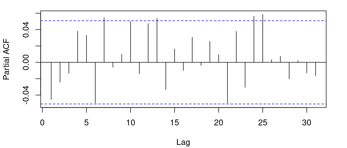
Take a look at the autocorrelation and partial autocorrelation for the Tata Steel returns.


The returns data do not have any significant autocorrelation (except at lag 0) or partial autocorrelation. This suggests that a constant mean or white noise model, ARMA(0, 0), would be appropriate.
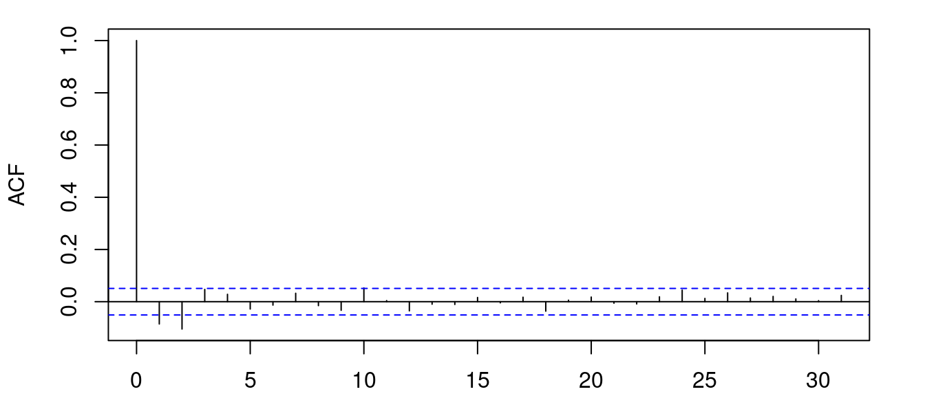
Somewhat surprisingly this appears to be the case for many of the returns time series. However, there are a few assets that do have significant autocorrelation or partial autocorrelation at non-zero lags. For example, Marico Ltd.


Here we can see (marginally) significant peaks at lags 1 and 2. Now a constant mean model is probably not the right choice.
specification <- ugarchspec(
  mean.model = list(armaOrder = c(1, 1)),
  variance.model = list(model = "sGARCH"),
  distribution.model = "sstd"
)

marico <- ugarchfit(data = MARICO, spec = specification)
Using the AR(1, 1) above we find significant estimates for both ar1 and ma1 model parameters.
round(marico@fit$matcoef, 3) Estimate Std. Error t value Pr(>|t|)
mu 0.001 0.000 1.917 0.055
ar1 0.459 0.124 3.692 0.000
ma1 -0.572 0.114 -5.032 0.000
omega 0.000 0.000 2.920 0.003
alpha1 0.154 0.045 3.432 0.001
beta1 0.586 0.117 4.998 0.000
skew 1.079 0.040 27.047 0.000
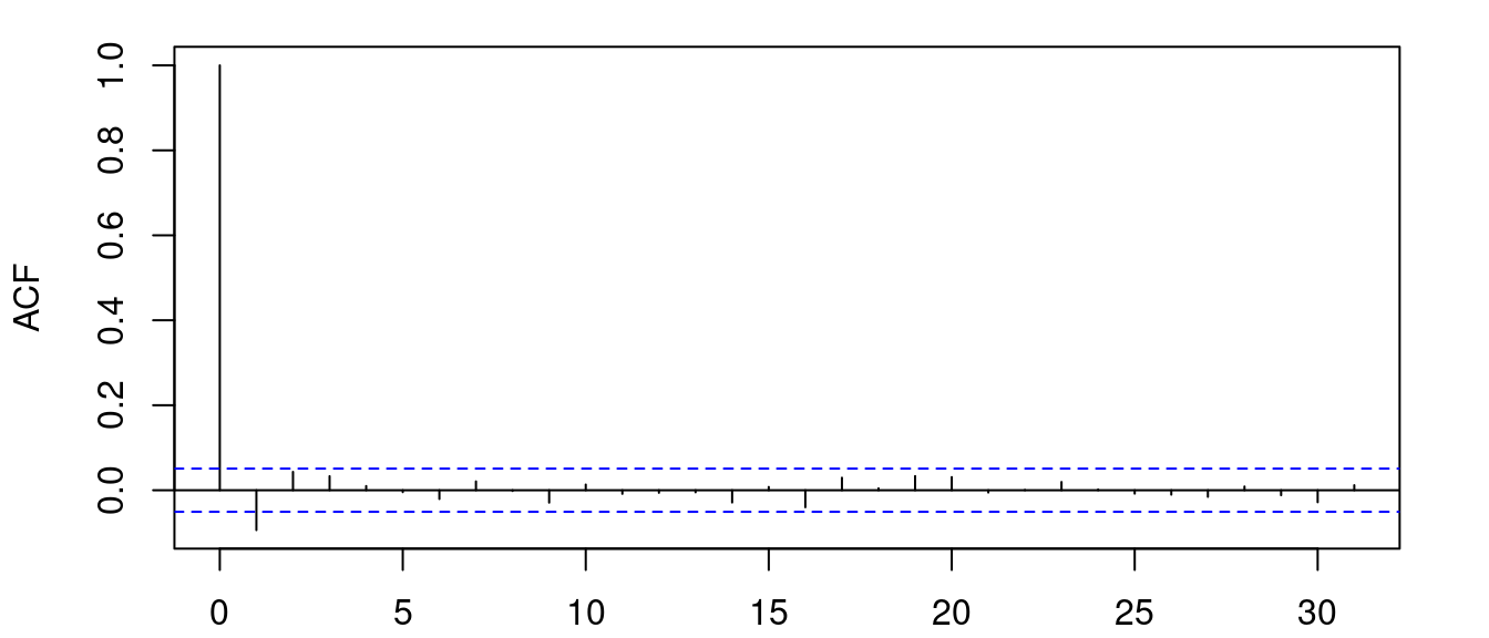
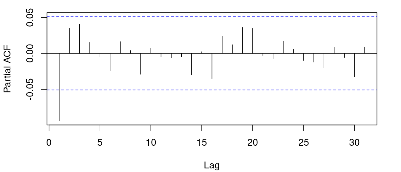
shape 4.897 0.614 7.970 0.000Things are not always that simple though. Here are the correlation plots for Titan Company Ltd.


There’s a (marginally) significant peak at lag 1. Now, although a constant mean model results in all model parameters being significant, attempting an AR(1), MA(1) or ARMA(1, 1) model gives significant estimates for the mean model but the omega estimate is no longer significant.
specification <- ugarchspec(
  mean.model = list(armaOrder = c(1, 0)),
  variance.model = list(model = "sGARCH"),
  distribution.model = "sstd"
)

titan <- ugarchfit(data = TITAN, spec = specification)round(titan@fit$matcoef, 3) Estimate Std. Error t value Pr(>|t|)
mu 0.002 0.000 3.582 0.000
ar1 -0.069 0.022 -3.115 0.002
omega 0.000 0.000 1.353 0.176
alpha1 0.033 0.018 1.903 0.057
beta1 0.919 0.049 18.947 0.000
skew 1.078 0.036 29.934 0.000
shape 3.196 0.293 10.893 0.000Once you start fiddling with these thing (and you should), it becomes apparent that it’s a rather deep rabbit hole and it can become somewhat confusing.
Alternative Implementation
Let’s try with the {tsgarch} package.
library(tsgarch)specification <- garch_modelspec(
TATASTEEL,
model = "gjrgarch",
distribution = "sstd",
constant = TRUE
)
fit <- estimate(specification)You don’t need to work as hard to examine the statistical properties of the parameter estimates: just use the summary() method.
summary(fit)GJRGARCH Model Summary
Coefficients:
Estimate Std. Error t value Pr(>|t|)
mu 1.281e-03 5.848e-04 2.190 0.02853 *
omega 7.364e-06 4.009e-06 1.837 0.06624 .
alpha1 1.051e-02 8.452e-03 1.243 0.21370
gamma1 5.787e-02 1.825e-02 3.171 0.00152 **
beta1 9.513e-01 1.263e-02 75.295 < 2e-16 ***
skew 1.054e+00 3.722e-02 28.307 < 2e-16 ***
shape 5.130e+00 7.007e-01 7.321 2.45e-13 ***
persistence 9.914e-01 7.208e-03 137.535 < 2e-16 ***
---
Signif. codes: 0 '***' 0.001 '**' 0.01 '*' 0.05 '.' 0.1 ' ' 1
N: 1484
V(initial): 0.0006137, V(unconditional): 0.0008568
Persistence: 0.9914
LogLik: 3492.33, AIC: -6968.67, BIC: -6926.25The AIC() and BIC() generic functions yield the Akaike (AIC) and Bayesian (BIC) Information Criteria.
AIC(fit)[1] -6968.666BIC(fit)[1] -6926.246Comparing these values to those obtained earlier it’s apparent that these metrics are being normalised differently, underlining the fact that they can only be used for making comparisons.