Geonode Proxies

Proxy services tend to make the same promises: global coverage, easy geo-targeting, sticky sessions and a dashboard full of connection strings. The useful questions are more prosaic. Can I get a working connection quickly? Do the exit IPs look plausible once I start sending real requests through them? How much additional latency does the proxy add?

After recently testing Massive’s residential proxies, I’m taking a look at Geonode. This isn’t a full benchmark. It’s a first pass at the things I want to know before using the service in a scraping workflow.

Here’s what I’ll cover:

• account setup, credentials and proxy configuration;
• smoke tests with curl and Python;
• a browser check to see rotating exits in practice;
• sampled exit locations, residential dispersion and ISP mix; and
• the latency overhead compared with direct requests.

Types of Proxies

Geonode’s docs describe the three proxy types they support:

• residential — broadband IPs from residential ISPs;
• datacentre — IPs from data centres (faster, less expensive, but also more likely to get blocked);
• mixed — a combination of residential and datacentre IPs.

Further details in the IP type documentation. I’ll focus on residential proxies (most useful for web scraping, which is what I care about).

Getting Started

I quickly created an account on Geonode and was itching to start exploring. Here’s a brief tour of the UI.

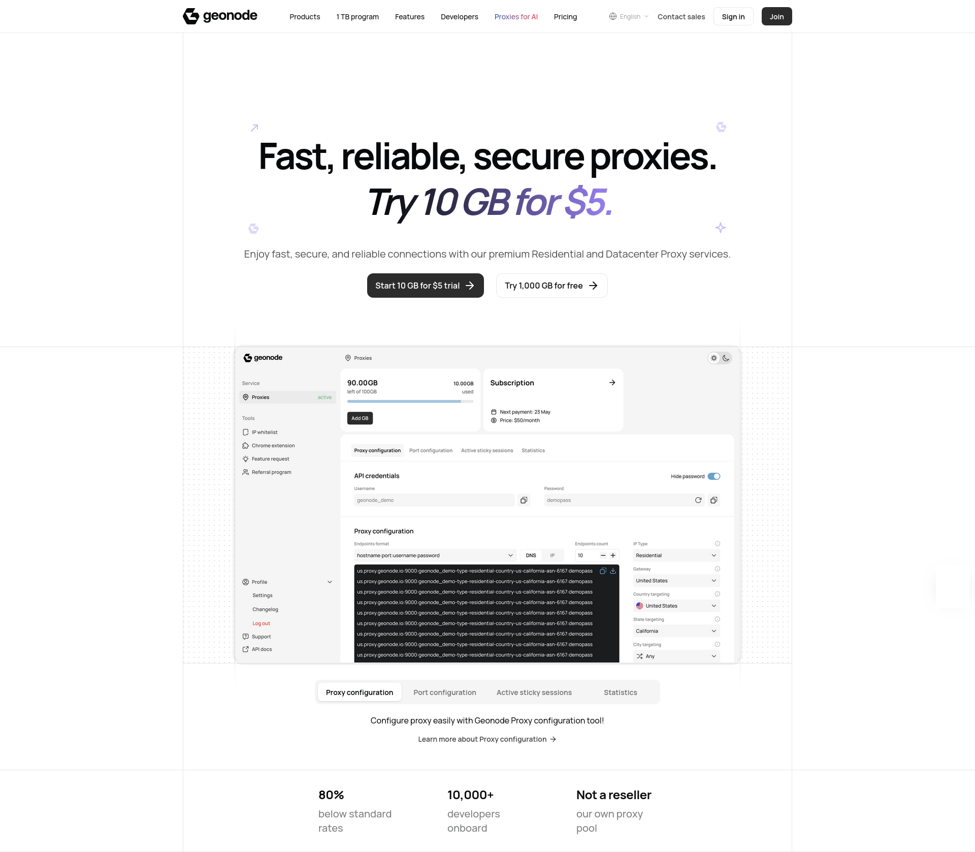
Landing Page

Go to the Geonode landing page at https://geonode.com/. It provides an overview of the service, links to their product and pricing pages as well as their documentation. It also includes an FAQ section that answers a few pertinent questions about the service, such as how subscriptions work and more details on features like geo-targeting and session management.

Geonode landing page.

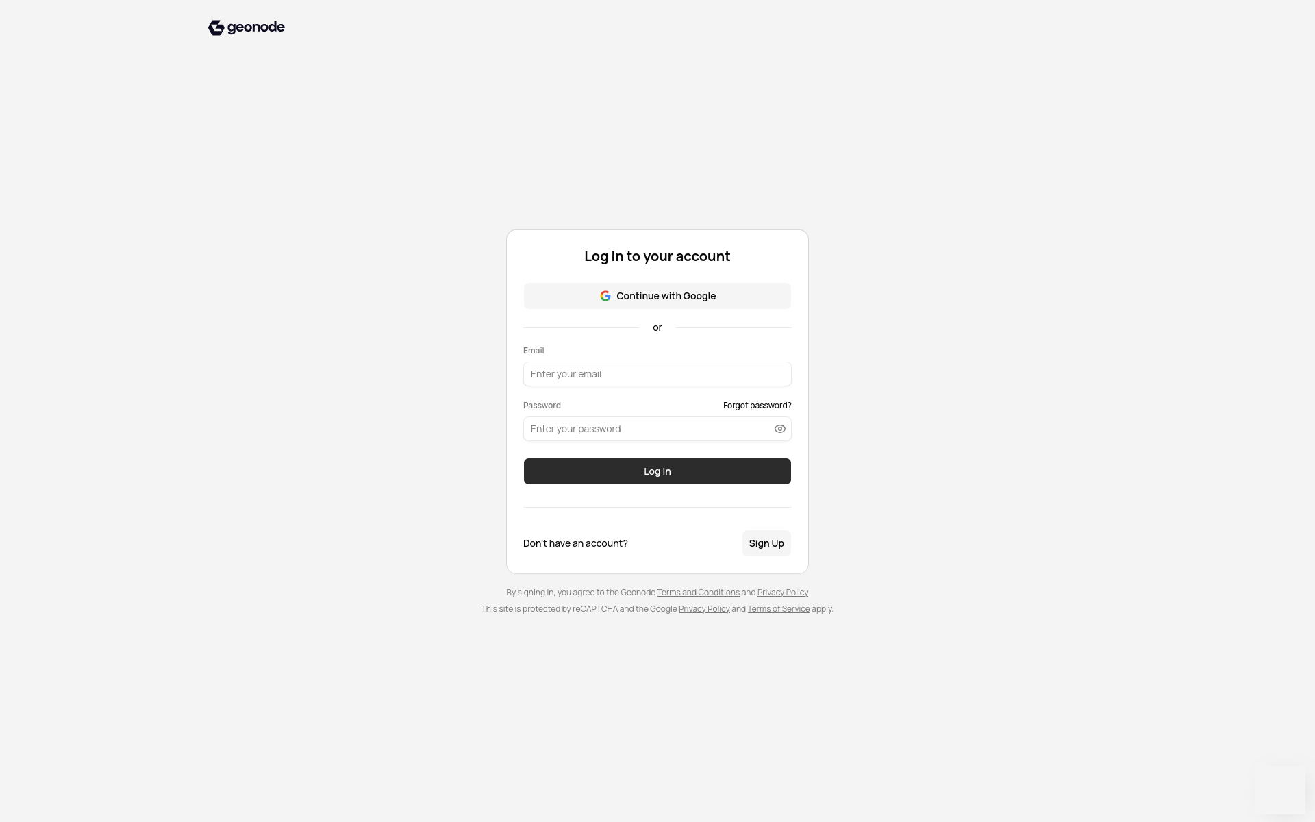
Login

Click the Sign In button or go directly to https://app.geonode.com/login. You can log in using a Google identity or an email address and password. Alternatively, click the Sign Up button to create an account. There’s a 5 USD trial or, if you are already a proxy power user, then sign up for the 1 TB program.

Geonode login page with email and password fields.

Dashboard

Once you’ve logged in you’ll see your dashboard. It provides quick access to the features in your account. You can generate proxy configurations for various combinations of parameters. There’s also a section that provides sample code for integration with various tools and languages, including curl, Python, Node.js, Java and Go.

Geonode dashboard page.

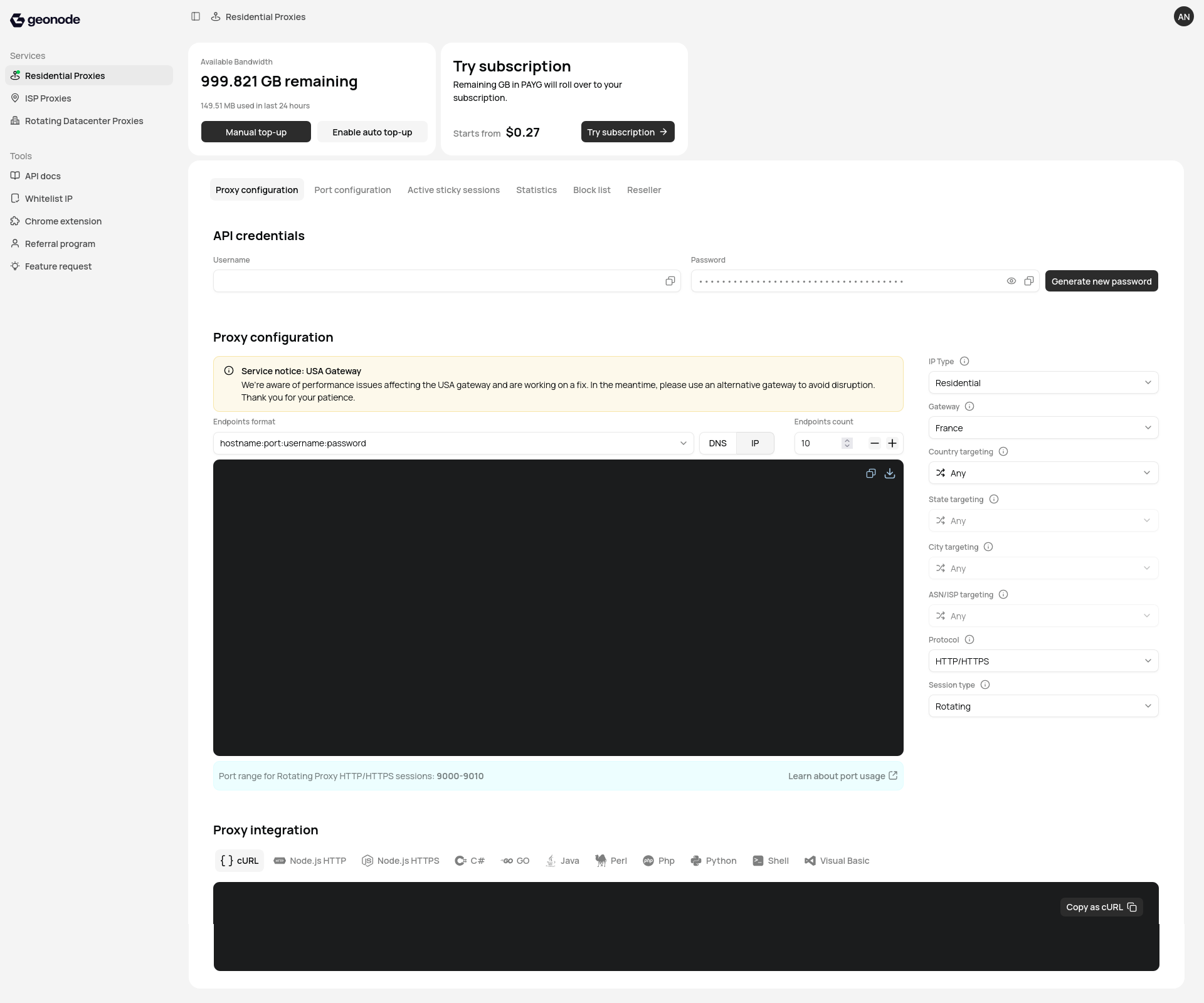
Your login credentials aren’t the same as your proxy credentials. Find the latter under API credentials on the dashboard. Use those when connecting to the proxy servers or you’ll spend quality time with (Proxy Authentication Required) errors, which is a dull way to lose ten minutes.

Your proxy username is fixed, but you can regenerate your proxy password on demand. Regenerating it will break existing scripts until you update their configuration. This is exactly what you want after a credential leak. But precisely what you don’t want five minutes before a scheduled job or a critical demo.

📌 You can whitelist your IP, after which you no longer need to provide credentials. I can see that this might be handy in some situations but I personally prefer to have granular control over my proxy usage.

Proxy Configuration

The Proxy configuration section on the dashboard is where you generate connection strings. Choose from a selection of different endpoint formats:

• hostname:port (presumably to be used with a whitelisted IP)
• hostname:port:username:password
• hostname:port@username:password
• username:password:hostname:port and
• username:password@server:port.

These options have limited utility. Normally I want each of these components separately rather than combined in a single string.

The remaining selectors are more useful.

The IP Type selector allows you to choose between the three proxy types (residential, datacentre and mixed). Specifying a proxy type adds a type segment to your username. There are also selectors for Country, State, City and ASN/ISP targeting. Each of those adds a corresponding segment to the username. ASN/ISP targeting is only available in conjunction with country targeting. Here are some examples of the additional username segments:

# Use datacentre proxies.
type-datacenter
# Use residential proxies in the UK.
type-residential-country-gb
# Use residential proxies in England (UK).
type-residential-country-gb-state-england
# Use mixed proxies in Chicago, Illinois (US).
type-mix-country-us-state-illinois-city-chicago
# Use residential proxies in Vodafone network in the UK.
type-residential-country-gb-asn-1273

The choice of Gateway determines the proxy host.

Gateway	Host
France	proxy.geonode.io
France (Whitelisted IP Only)	prod-proxy.geonode.io
United States	us.proxy.geonode.io
Singapore	sg.proxy.geonode.io

The Protocol and Session Type (rotating or sticky) selectors determine the port:

• HTTP(S) — 9000 for rotating sessions and 10000 for sticky sessions; and
• SOCKS5 — 11000 for rotating sessions and 12000 for sticky sessions.

📌 Those ports are actually the anchors for port ranges. For example, a rotating HTTP(S) proxy is available on ports 9000 to 9010. There’s more in the port usage documentation.

Smoke Test

The Proxy integration section on the dashboard provides sample code for testing your proxy connection. The code updates with the selections made under Proxy configuration.

Here’s an example of a curl command sending a request to http://ip-api.com without providing specific proxy configurations.

curl -x proxy.geonode.io:9000 -U "******:******" http://ip-api.com

I’m using ******:****** to represent my username and password. Don’t forget to replace those with your proxy credentials.

The response informs me that the request was routed via an IP in Kokshetau, Kazakhstan (definitely not my actual location!) using the JSC Kazakhtelecom ISP (AS9198) network.

{
  "status"       : "success",
  "continent"    : "Asia",
  "continentCode": "AS",
  "country"      : "Kazakhstan",
  "countryCode"  : "KZ",
  "region"       : "11",
  "regionName"   : "Aqmola",
  "city"         : "Kokshetau",
  "district"     : "",
  "zip"          : "",
  "lat"          : 53.2852,
  "lon"          : 69.3922,
  "timezone"     : "Asia/Almaty",
  "offset"       : 21600,
  "currency"     : "KZT",
  "isp"          : "JSC Kazakhtelecom",
  "org"          : "JSC Kazakhtelecom",
  "as"           : "AS9198 JSC Kazakhtelecom",
  "asname"       : "KAZTELECOM-AS",
  "mobile"       : false,
  "proxy"        : false,
  "hosting"      : false,
  "query"        : "37.150.123.115"
}

Here’s some code generated for Python. I explicitly specified a residential proxy and that’s reflected in the username.

#!/usr/bin/env python3

import requests

username = "******-type-residential"
password = "******"
GEONODE_DNS = "proxy.geonode.io:9000"
urlToGet = "http://ip-api.com"
proxy = {"http":"http://{}:{}@{}".format(username, password, GEONODE_DNS)}
r = requests.get(urlToGet , proxies=proxy)

print("Response:\n{}".format(r.text))

That works perfectly too. Although I would have used httpx. Just a personal preference.

Browser Check

I normally use proxies for automation, but from time to time I also use them in the browser. It’s also a good test of the proxy’s real-world performance and reliability. I configured my browser to use the proxy host and port. Then navigated to https://whatsmyip.com/. The browser prompted me for username and password, which I provided.

What’s My IP page showing a proxy exit IP address located in Managua, Nicaragua.

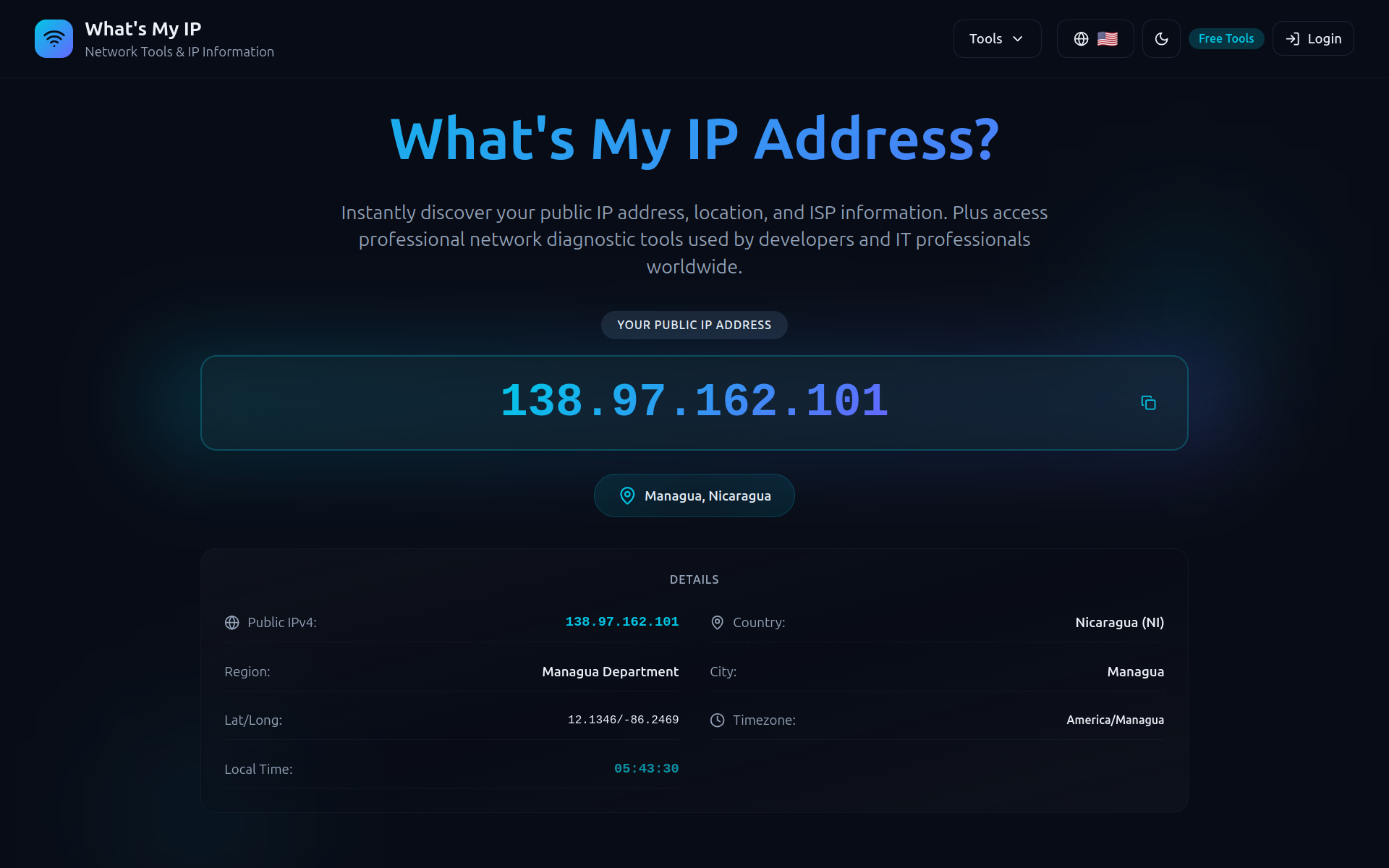
Suddenly I’m in Nicaragua! Well, at least as far as the internet is concerned.

What’s My IP page showing a proxy exit IP address located in Rancagua, Chile.

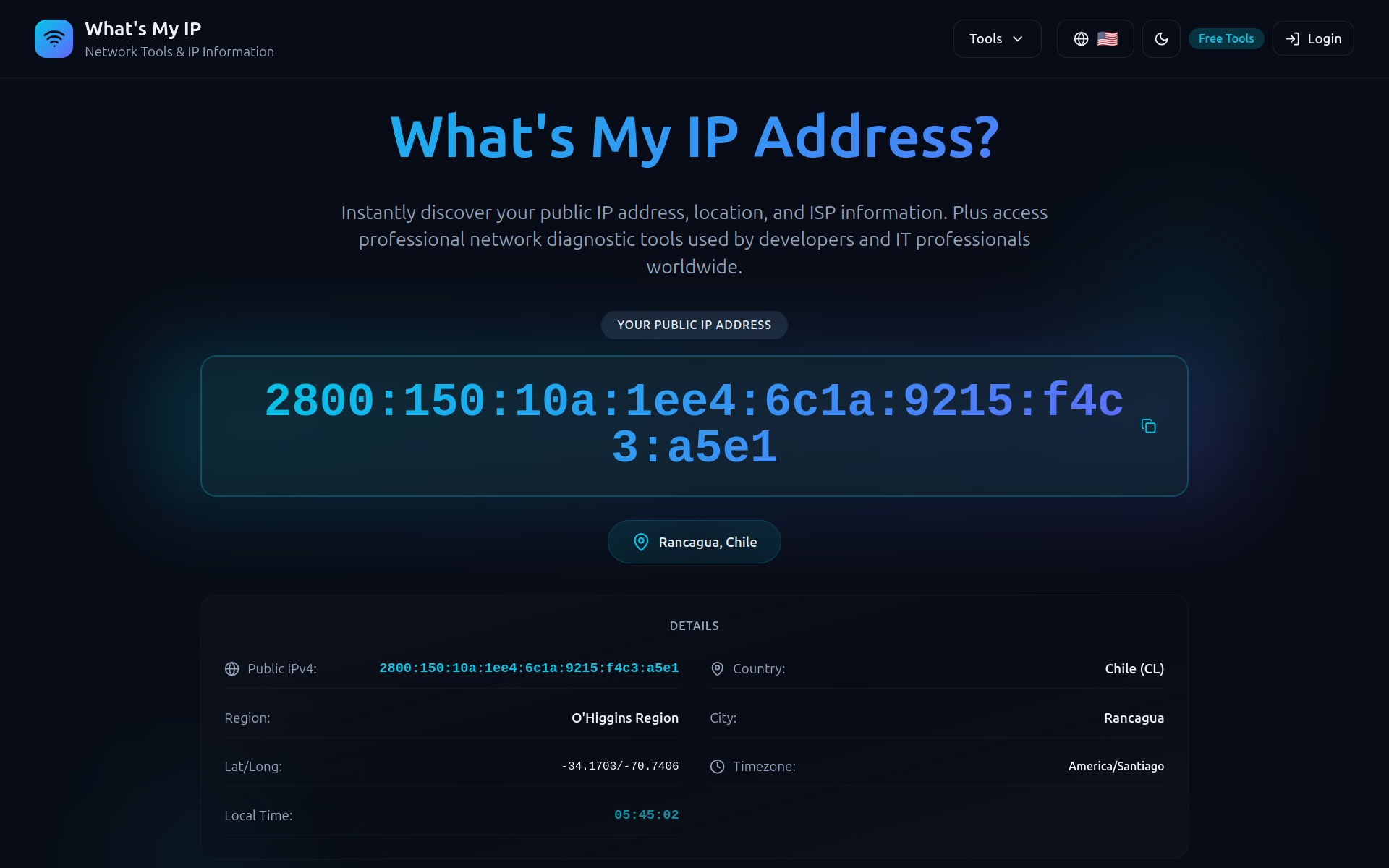
But on the next request I’m in Chile! If only travel were this easy. Interesting to see both IPv4 and IPv6 exits in the mix.

How Good Is It?

For an initial assessment of the residential proxy service I set out to answer two questions:

1. What’s the geographic distribution of the exit IPs?
2. How does the proxy impact response times?

Geographic Distribution

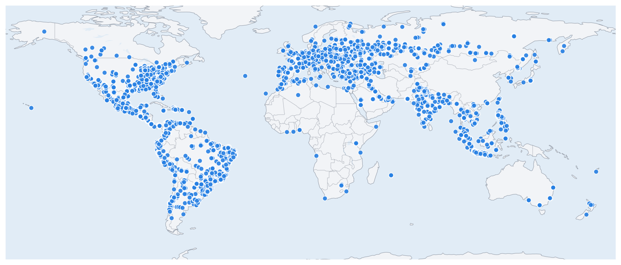
I used the Geonode proxies to gather the responses from 5,000 requests to http://ip-api.com. Each response contains the geographic location, country, city and postal code of the proxy exit IP. The results are recorded in a JSONL file. The plot below shows the locations of the sampled exit IPs.

Figure 1: Observed proxy exit points.

The overall distribution of exit IPs is impressive. Good coverage in North and South America, Europe and Asia. A few locations in Africa and Australia as well. Nothing in Antarctica though. What’s up with that? 😜

Geonode’s geographic coverage appears more extensive than that of Massive.

Residential Locations

Are the exit IPs actually in residential locations? It’s hard to provide a definitive answer. But we can use the cities and postal codes from the http://ip-api.com/ geolocation data as a proxy. If the exit IPs are clustered in a few cities or postal codes then that would be a sign of datacentre proxies masquerading as residential ones. On the other hand, if the exit IPs are spread across many cities and postal codes then that’s a good indicator of residential dispersion.

The plot below shows the proportion of distinct cities and postal codes relative to the sample size. The data are broken down by country and ordered by postal code coverage. To keep the chart readable it excludes countries with fewer than 20 samples. Faded dots quantify cities or postal codes missing from the geolocation data.

Figure 2: Distinct cities and postal codes relative to sample size, with faded dots showing missing city and postal-code data.

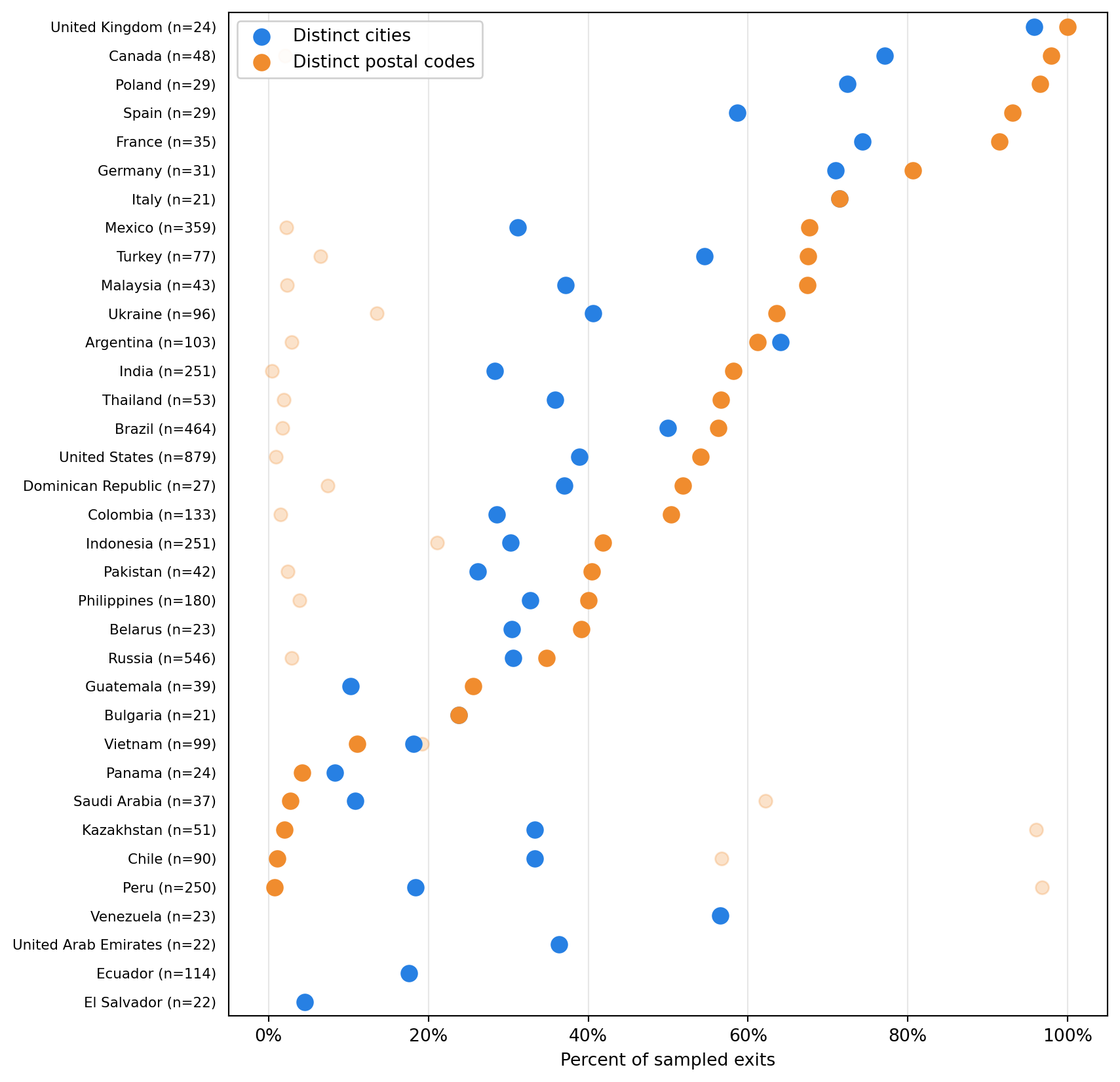
Most countries show dispersion in both city and postal code coverage. Ideally we’d like to see 100% distinct cities and postal codes, but that’s not realistic with this sample size. Some exit IPs will inevitably cluster in the same city or postal code. The samples were spread across 114 countries, with 1,866 distinct country-city and 2,232 distinct country-postal code combinations, which is promising. It suggests that the exit IPs aren’t clustered in a few locations but spread across many different ones, which is what we’d expect from residential proxies.

What about ISPs? The plot below shows the ranking of ISPs (also provided by http://ip-api.com/ geolocation data). To keep the ISP ranking focused on providers with enough observations to be meaningful, the chart excludes providers with fewer than 20 samples.

Figure 3: Reported ISPs among the sampled exits, excluding providers with few samples.

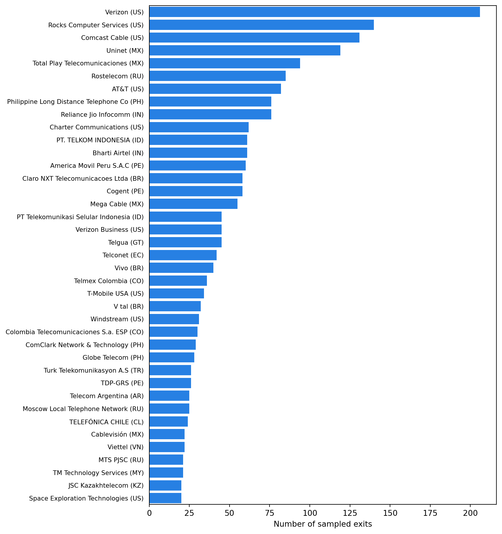
If the list of ISPs was dominated by a few corporate-sounding names then that would be a sign of datacentre proxies masquerading as residential ones. This is certainly not what we see! The heavy hitters, Verizon (206), Rocks Computer Services (140), Comcast Cable (131), Uninet (119) and Total Play Telecomunicaciones (94), are all recognisable consumer providers. There are a few labels that sound slightly more corporate than domestic, like Verizon Business, but they still belong to ordinary connectivity providers rather than obvious datacentre hosts.

Direct Versus Proxy Timing

To assess the latency overhead of the proxy, I also collected timing data for 5000 matched pairs of requests to 25 distinct URLs across 14 domains. The same URL was requested once directly and once through the proxy, with both requests sent simultaneously. The results are recorded in a JSONL file. Direct requests averaged about 99 ms and proxied requests around 1,716 ms. Proxied requests are relatively slow. But that’s expected.

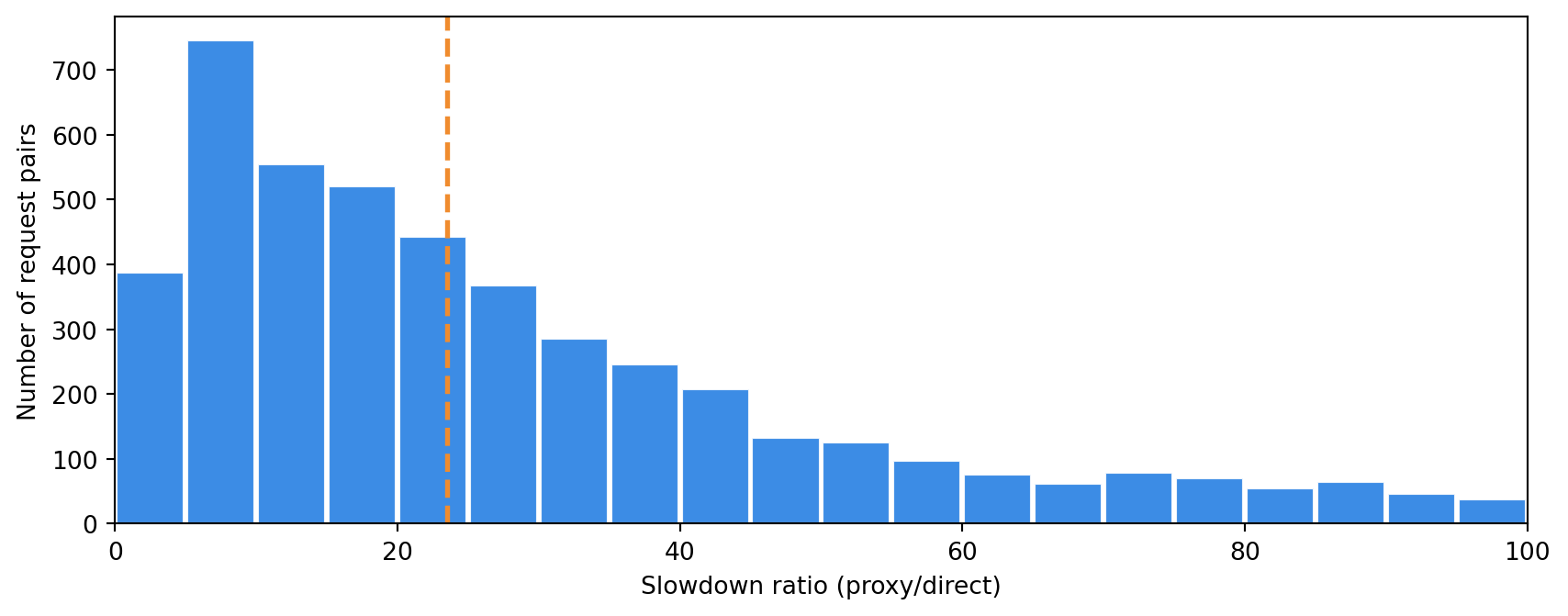
The plot below displays the distribution of slowdown ratios, calculated as proxy time divided by direct time. The vertical dashed line indicates the median slowdown ratio of about 23.5. This view is intuitive, but it can be misleading when the direct request is very fast.

Figure 4: Distribution of slowdown ratios, calculated as proxy time divided by direct time. The vertical dashed line indicates the median slowdown ratio.

Rather than multiplying the direct request time, the proxy is more likely to add latency on top of the direct request time. The plot below shows the added latency in milliseconds, calculated as proxy time minus direct time. The horizontal dashed line indicates the median of about 1,249 ms. Both axes are logarithmic so that the slower requests do not completely dominate the picture.

Figure 5: Proxy overhead versus direct time on logarithmic axes. The horizontal dashed line indicates the median added latency.

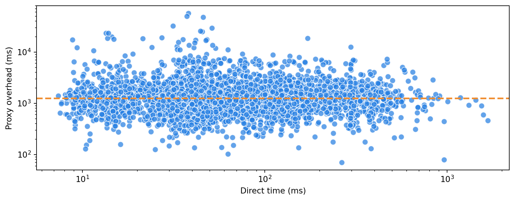
The distribution of the proxy overhead appears to be independent of the direct request time, which supports the additive model. It also means that the direct time axis in the previous plot isn’t informative. The plot below simply shows the distribution of proxy overhead values, which are clearly peaked around the median.

Figure 6: Distribution of proxy overhead values on a logarithmic x-axis. The vertical dashed line indicates the median added latency.

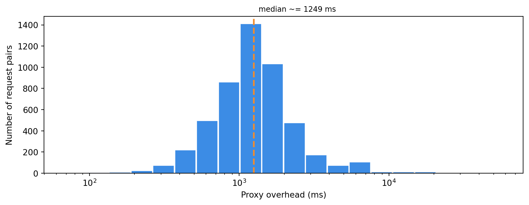
The median overhead of 1,249 ms is slightly higher than the overhead I observed for Massive. That may simply be the trade-off for the broader coverage in South America and Asia.

Finally, comparing the median direct and proxy times for the top domains in the sample can help us understand whether the slowdown is consistent across sites or if a few hostnames dominate the results.

Figure 7: Median direct and proxied timings by target domain on a logarithmic scale.

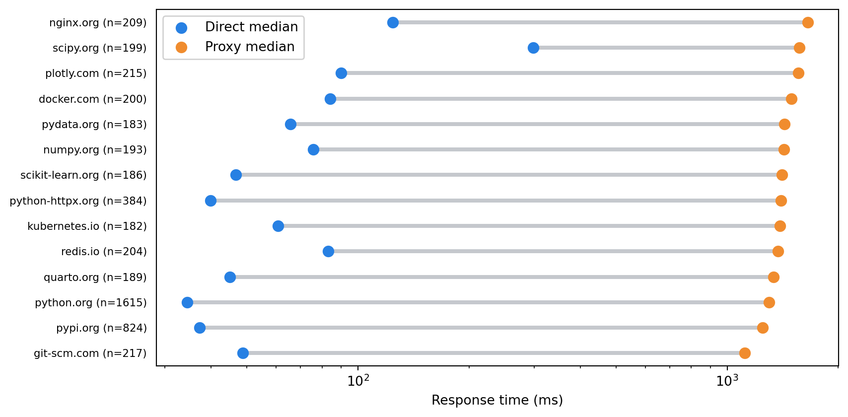
The direct response times indicate that there are “fast” and “slow” sites in the sample. However, once the proxy overhead is added, the response times are more uniformly distributed (at least in a logarithmic sense). The slowdown appears to be consistent across sites, with no obvious outliers.

Summary

Geonode ticks the important boxes for a residential proxy service. Quick setup. Sensible controls. The exit IPs were geographically distributed and the ISP mix looks credible. The proxy overhead was non-negligible, but consistent and predictable. That’s a practical combination.

For the kind of scraping workflow I care about, Geonode looks eminently usable.