The Thames 200 Ultra is a 200 km event on the River Thames from Lechlade to Teddington. It’s now in its third year and I have enjoyed (for certain values of “enjoy”) being on a Newbury Canoe Club relay team for the last two years.
Entries are divided into three categories:
- double (two people covering the full distance)
- individual (one person covering the full distance)
- relay (split the distance into six legs with different people doing one or more legs each).
The race has six legs punctuated by Check Points (CPs):
- Start (Lechlade)
- CP1 (New Bridge, 26.5 km, 6 portages)
- CP2 (Abingdon, 37.0 km, 9 portages)
- CP3 (Pangbourne, 36.5 km, 7 portages)
- CP4 (Bisham, 37.5 km, 8 portages)
- CP5 (Staines, 35.0 km, 8 portages)
- Finish (Teddington, 27.5 km, 6 portages). Effectively CP6.
Each leg has its own set of challenges. Some have more portages; others start and/or end in the dark.
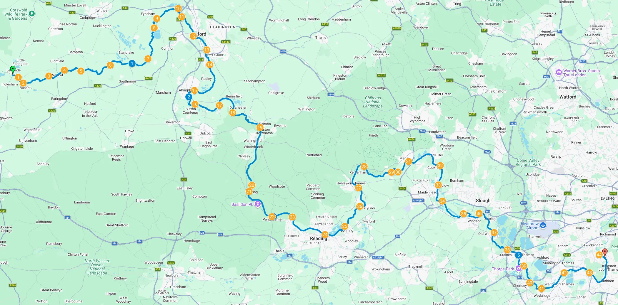
The race presents a massive physical challenge. But it’s also logistically tough for spectators and supporters. The support for relay teams is particularly daunting. Whether you’re a competitor, spectator or supporter you need to work out the expected times at various locations along the route.
The published results for each entry include times for each CP and the finish. This presents an opportunity to build a model to predict times based on data from previous years.
Acquiring the Data
I scraped the published results and dumped them to a series of JSON files:
- 2024 results (23 finishers)
- 2025 results (29 finishers) and
- 2026 results (40 finishers).
The volume of data is limited: only 92 finishers in total, broken down by category as 61 relay, 21 individual and 10 double.
Building a Model
Modelling the race is interesting for a couple of reasons:
- the differences between legs (distance and number/type of portages) and
- double/individual paddlers going the full distance versus relay entries changing paddlers between legs.
A Bayesian model is a natural fit due to the limited data available and because uncertainty will be a vital component of any predictions. The Bayesian approach lets the model pool evidence across races, starting with a category-specific baseline and updating predictions as checkpoint times are added.
If you’re not interested in the technical details then skip forward to the results.
Let \(t_{ij}\) be the time for entry \(i\) on leg \(j\). Rather than modelling the times, \(t_{ij}\), we’ll model the logarithm of the times, \(y_{ij} = \log t_{ij}\). The model output is then transformed to \(\exp y_{ij}\), which is linear and can be added to create cumulative times. Modelling the logarithms has some advantages:
- times tend to vary proportionally rather than additively (comparing one leg to another, it’s more likely to be 10% slower than 5 minutes slower);
- enforces positive times; and
- produces asymmetric (right-tailed) uncertainties when converted back to linear space.
The paddlers in a double/individual entry are the same throughout the race, while those in a relay entry vary from leg to leg. For a double/individual entry a fast time at CP1 is an indication of fast paddlers and should strongly influence predictions for later in the race. A fast time for CP1 in a relay entry only tells us that the paddlers for the first leg were fast; it says much less about the paddlers for later legs (although there are other factors, like general team quality, boat, support and experience). This is borne out by the correlations between split times, which is ~0.9 for double/individual and ~0.7 for relay entries. To build this into the model, each entry uses either the continuous crew type (individual and double) or the relay crew type.
The model fits the \(y_{ij}\) to a Student-t distribution, \(\mathcal{T}\), with four degrees of freedom:
\[ \begin{aligned} y_{ij} &\sim \mathcal{T} (\alpha_j + \gamma_c + u_i,\ \sigma_j) \\ u_i &\sim \mathcal{N}(0,\ \tau_g) \end{aligned} \]
where
- \(i\) indicates a specific entry;
- \(j\) denotes a particular leg (1 to 6);
- \(c\) is the category for entry \(i\) (either
double,individualorrelay); - \(g\) is the crew type for entry \(i\) (either
continuousorrelay); - \(\alpha_j\) is the baseline log time for leg \(j\);
- \(\gamma_c\) is the effect of category \(c\);
- \(u_i\) is the entry’s shared latent pace, which captures the inherent speed of entry \(i\) (a positive value makes all six legs slower, while a negative value makes them faster);
- \(\tau_g\) controls how much shared pace varies between entries of crew type \(g\); and
- \(\sigma_j\) is the residual variation on leg \(j\).
The category effect is a shared adjustment for all entries in a particular category. For example, a positive category effect for relay would mean that relay entries should take (proportionally) a little longer on each leg relative to the overall average, while a negative category effect would mean the opposite. This is the shared tendency of all entries in a specific category (for example, all relay entries are 10% slower than average). The category effects are centred to sum to zero, keeping the baseline as the average leg profile.
The latent pace, \(u_i\), captures the pace of a particular entry. This explains why a specific entry in a particular category is faster or slower than the other entries in the same category. The model learns separate shared-pace variation, \(\tau_g\), for continuous crews and relays. It keeps one residual variation term for each leg, \(\sigma_j\), across both types. This is a deliberate simplification: the data can support different between-leg correlations for the two crew types, but not a stable collection of twelve separate crew-type-by-leg residual scales.
To predict a new entry, the model first creates complete timetables for all legs from its category, crew type and an unknown pace. It converts the six simulated log-splits back to hours and adds them to obtain cumulative checkpoint times. The initial forecast consists of thousands of plausible, internally consistent timetables.
At the start, no observed times constrain that timetable, so the forecast is simply the category-conditioned distribution. Once a checkpoint time is supplied, the model updates the entry’s latent pace and, through that pace, the distribution of later legs. The observed checkpoint effectively acts as a soft filter: timetables compatible with the observation receive more weight, while incompatible ones receive very little. The remaining weighted timetables form the updated forecast.
The model uses NUTS (No U-Turn Sampler), a Hamiltonian Monte Carlo sampler, via PyMC to sample the posterior distribution. A standard prediction run uses four chains, each with 1000 warm-up draws and 1500 retained draws. That produces 6000 simulated but internally consistent target timetables. An early CP3 and early finish in the same draw stay connected, rather than being assembled from unrelated checkpoint intervals.
The model output reports a median and distribution of times at each checkpoint. A broad distribution means that the results have a wide range of plausible times. Conversely, a narrow distribution indicates a higher level of confidence.
Results
Let’s consider a variety of hypothetical applications of the model. To make the results easier to compare it’s assumed that all categories start the race at the same time of day, 14:00. All of the checkpoint times used here are fictional and used for illustration only.
Start
What is the distribution of likely checkpoint times at the start? Since none of the entries have reached the first checkpoint, there’s no additional data to refine the predictions. All entries in a particular category are considered the same (although in practice this is patently not true!). Strictly, these are category-conditioned posterior baselines.
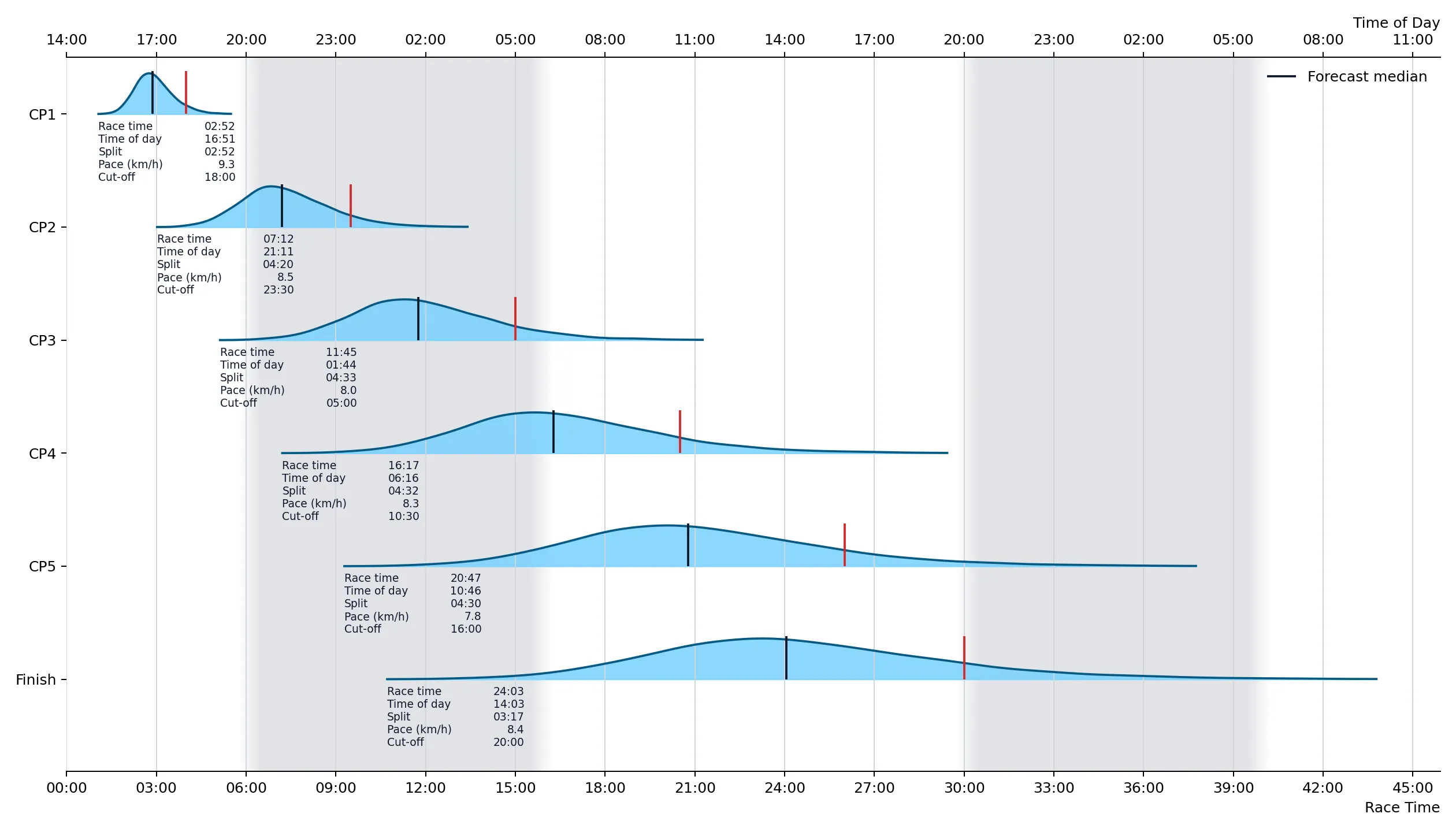
The plot below shows the expected arrival times at each of the checkpoints and finish for an “average” entry in the double category. It does not take into account the performance of any specific entry during the race. Without further information it’s expected that a double entry should finish the race in around 24.0 hours. Because we don’t know anything specific about the entry (yet!) the predicted distribution of times is broad at all of the checkpoints.
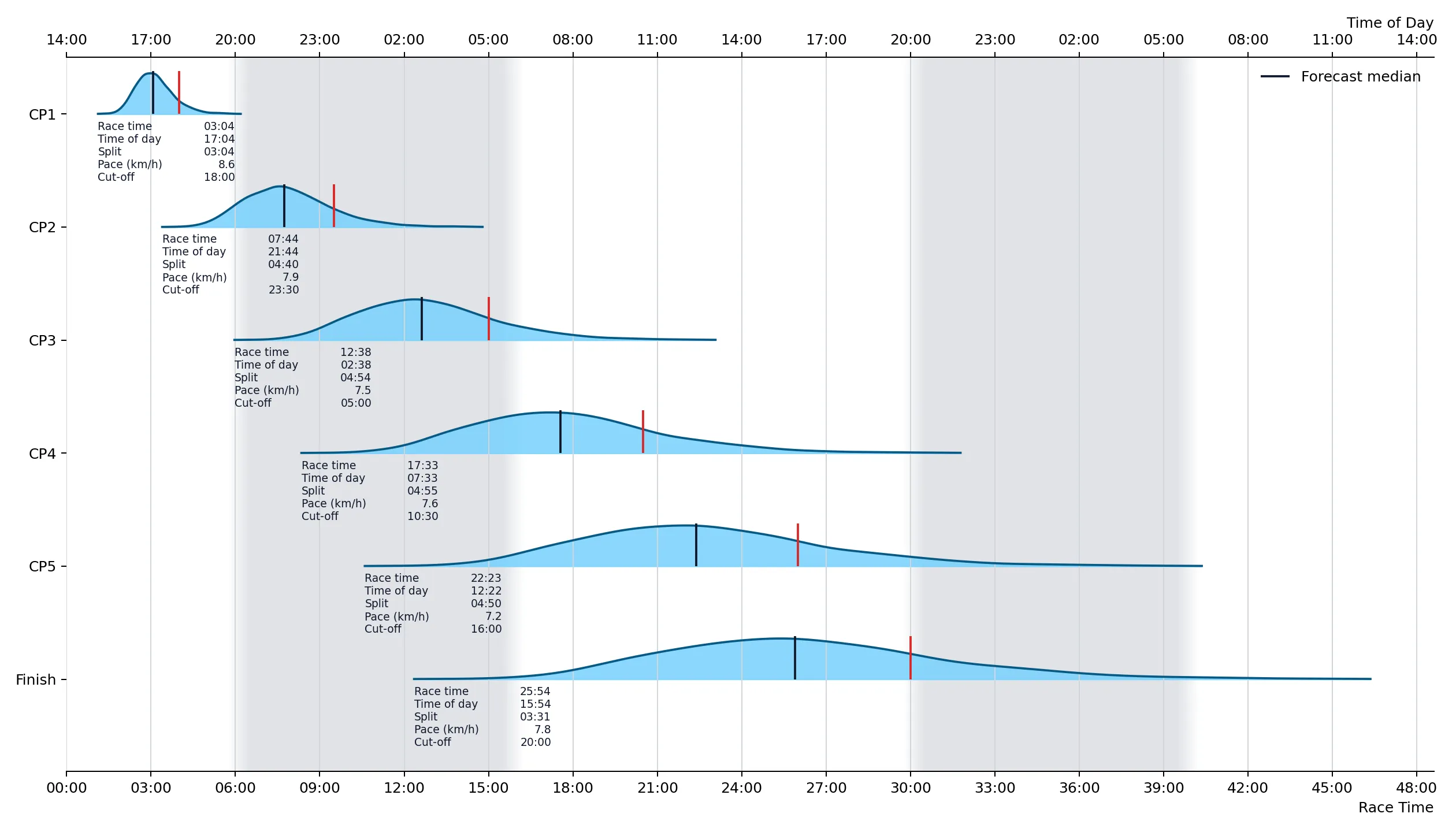
The distribution of predicted times at the start for an “average” individual entry is similar, but the expected finish time shifts back to around 26 hours, consistent with the fact that the power generated by two bodies is generally greater than that from one.
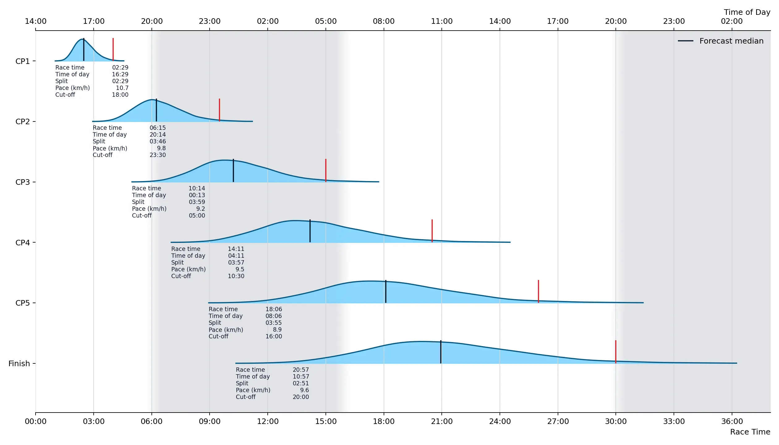
Finally, consider the predictions for an “average” relay team. The expected finishing time shifts forward to about 21 hours (consistent with the fact that the overall race has consistently been won by a relay team) but the distribution of times is broader due to the greater level of performance uncertainty associated with these teams.
It’s interesting to look at the median predicted pace for each of the legs broken down by category.
| Leg | km | Portages | Double | Individual | Relay | |||
|---|---|---|---|---|---|---|---|---|
| 1 | Start | — | CP1 | 26.5 | 6 | 9.3 | 8.6 | 10.7 |
| 2 | CP1 | — | CP2 | 37.0 | 9 | 8.5 | 7.9 | 9.8 |
| 3 | CP2 | — | CP3 | 36.5 | 7 | 8.0 | 7.5 | 9.2 |
| 4 | CP3 | — | CP4 | 37.5 | 8 | 8.3 | 7.6 | 9.5 |
| 5 | CP4 | — | CP5 | 35.0 | 8 | 7.8 | 7.2 | 8.9 |
| 6 | CP5 | — | Finish | 27.5 | 6 | 8.4 | 7.8 | 9.6 |
Those values do not describe the pace of any one entry, but are based on an aggregate of all entries in a category. They can be interpreted as saying something about the legs themselves.
- Leg 1 — Fastest for all categories. It’s the shortest leg (26.5 km) and has only 6 portages. Paddlers are fresh (more important for double/individual entries). Daylight.
- Leg 2 — Appreciably slower. Longer (37.0 km) with 9 portages (the most in any leg). Daylight, dusk and into the night.
- Leg 3 — Even slower. Comparable distance (36.5 km) but with only 7 portages. Dusk and night.
- Leg 4 — Slightly faster despite being fractionally longer and with 8 portages. Night and dawn.
- Leg 5 — Slowest for double and individual entries. Dawn and daylight.
- Leg 6 — Faster than previous leg for all categories (it’s the last leg! 💥). Shorter and fewer portages. Dawn and daylight.
Relay
If you were planning the handover and support schedule for a relay entry, then the estimated checkpoint times from before the start would probably be a useful guideline. But if you know the capabilities of the paddlers, then you could probably do better by making simple estimates in a spreadsheet.
This is true only until you have an observed time for the first checkpoint. Suppose that the first crew reached CP1 in 02:45. Adding this information immediately updates the median estimates for the remaining checkpoints and compresses the associated uncertainties.
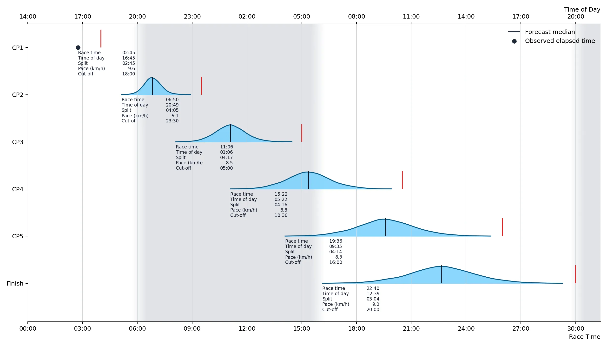
If the next three checkpoint times are 07:00, 10:40 and 14:30, then we have fairly precise predicted times for CP5 and the finish.
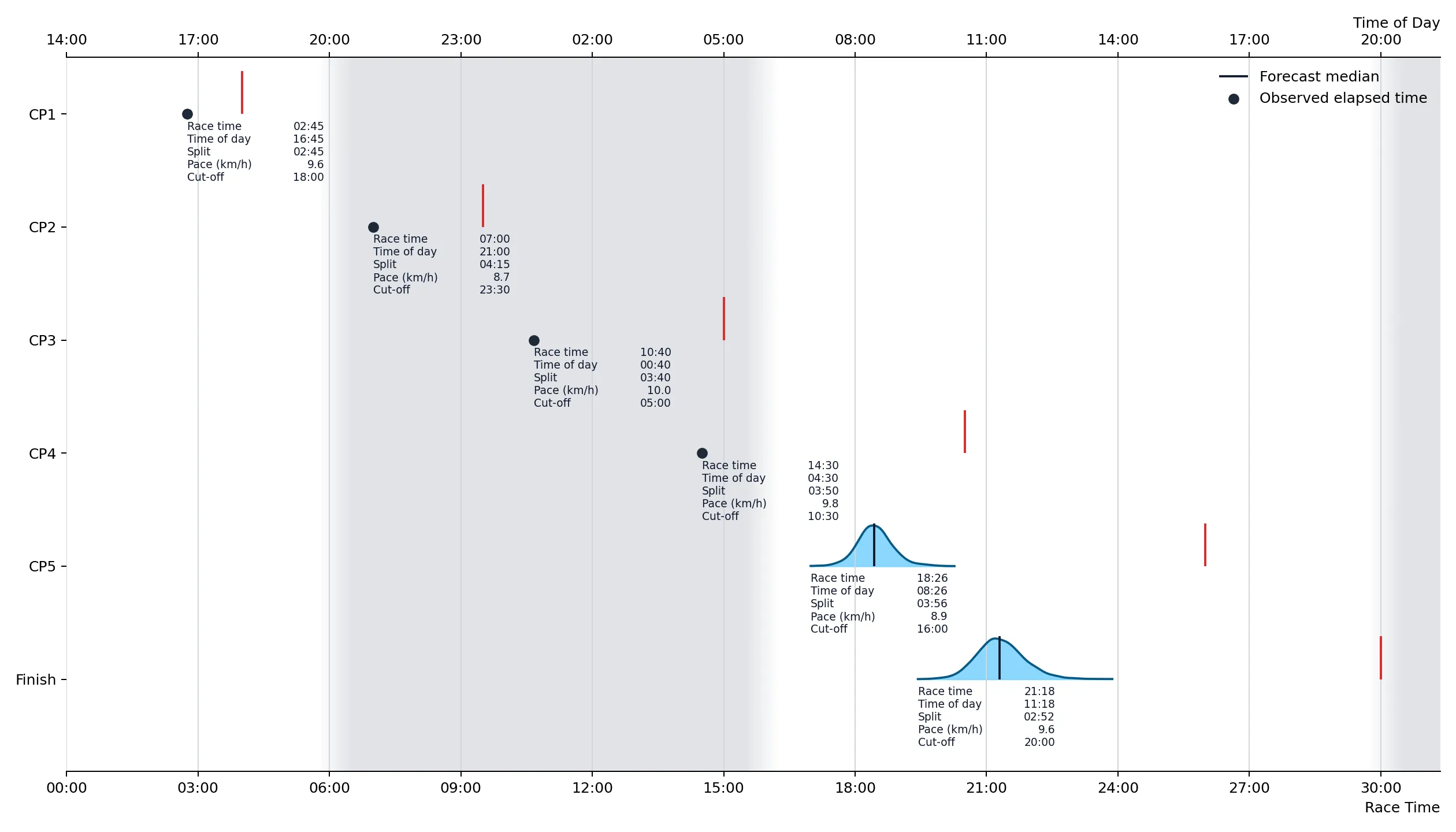
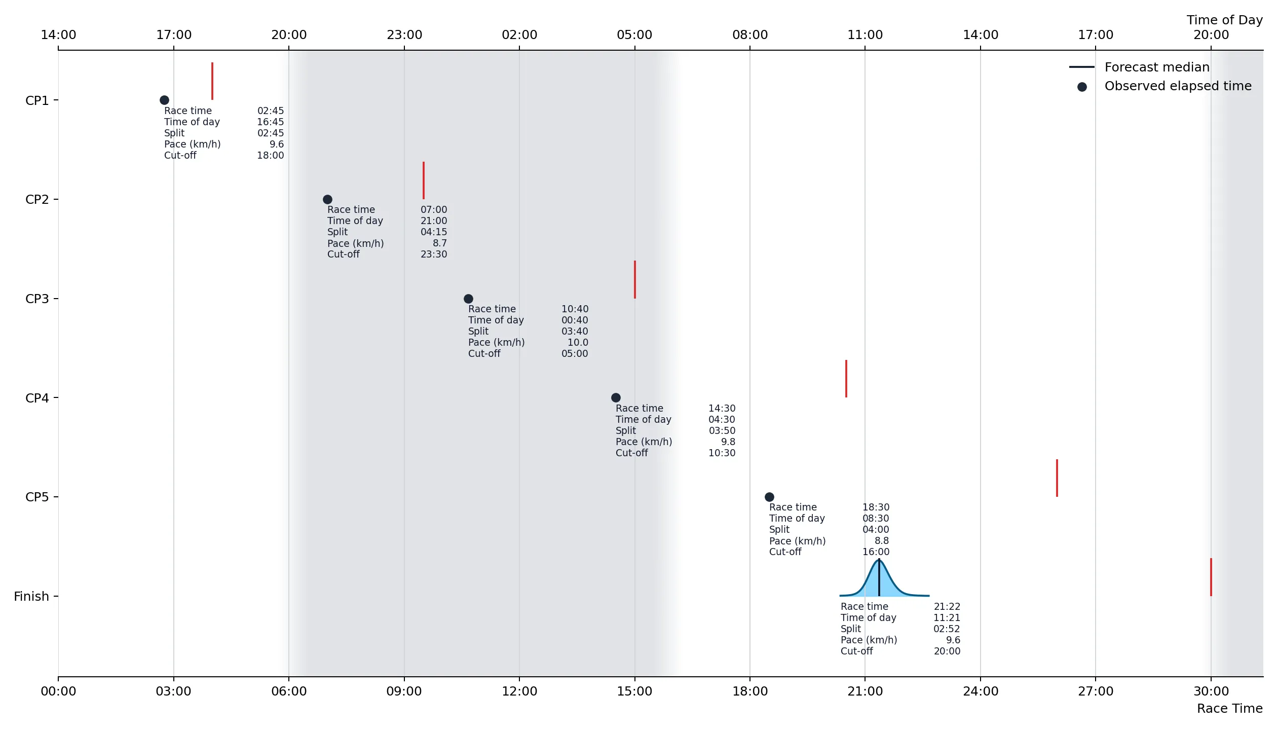
If the observed time for CP5 is 18:30, close to the predicted time, then there’s a small adjustment to the predicted finish time and the range of uncertainty shrinks even further.
Double
Let’s consider a case where something goes seriously awry during the night. Suppose that a double entry has solid times for the first three legs.
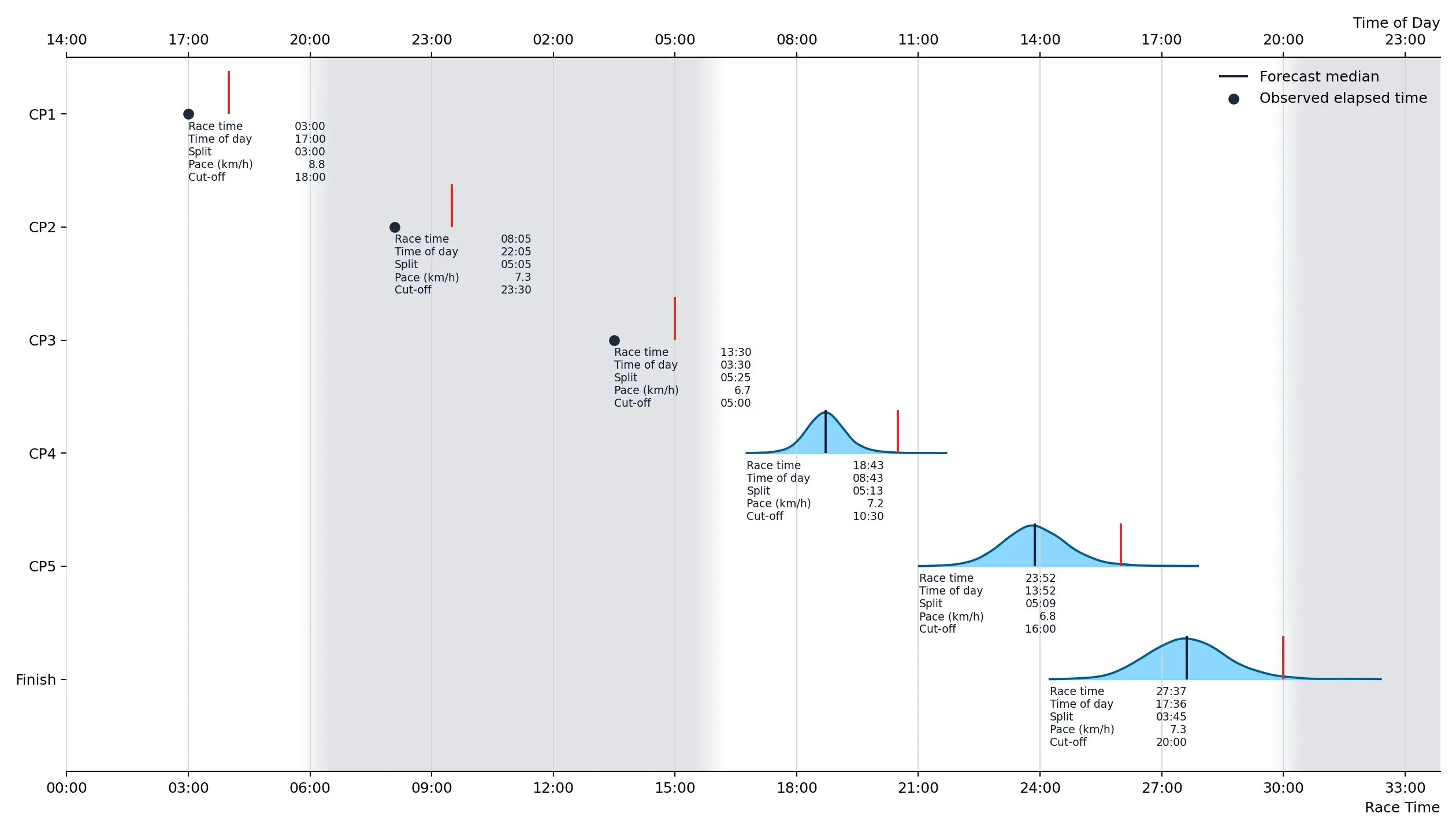
During the fourth leg they suffer the triple misfortune of having a swim, taking a detour down a dead end and getting a broken rudder. Combined, these issues set them back by at least 90 minutes, so that rather than getting to CP4 in 18:43, they only arrive in 20:20, putting them perilously close to the cutoff. The model predicts that if they can get back onto a similar pace to previous legs, then they’d still be on track for a strong finish.
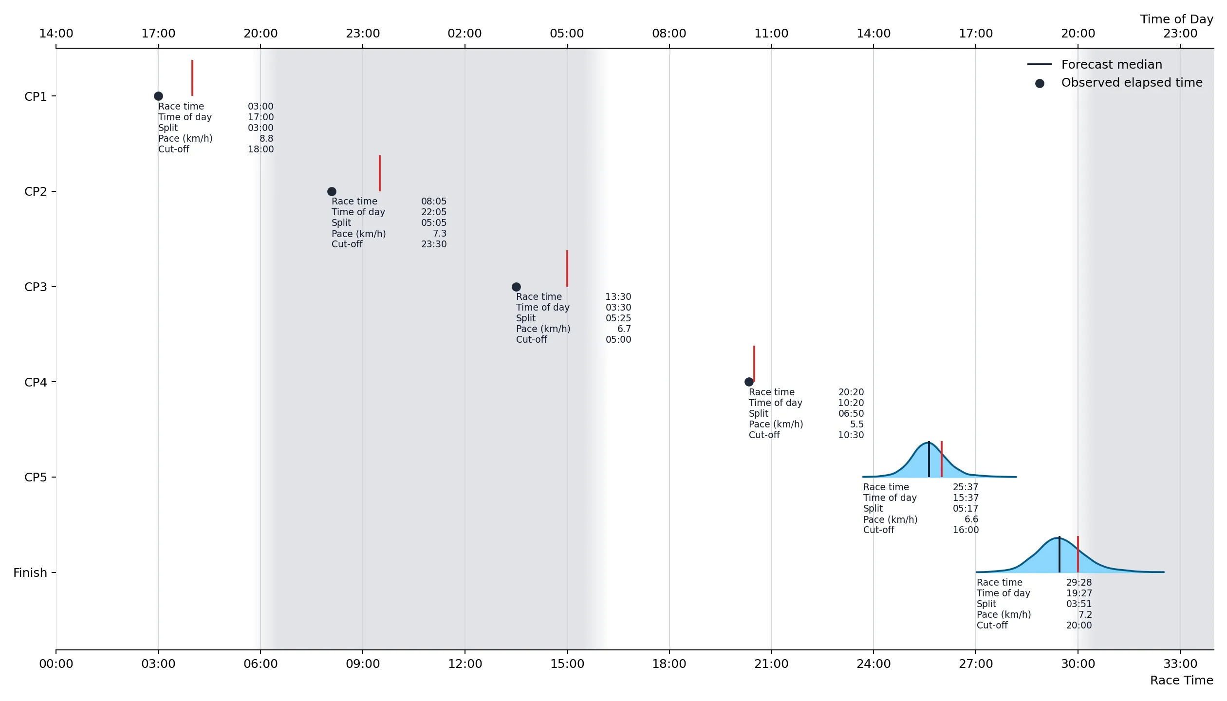
Obviously they got a serious pep talk from their support crew because they were back in the game on leg 5, with a split of 05:00, moving their predicted finish time away from the final cutoff.
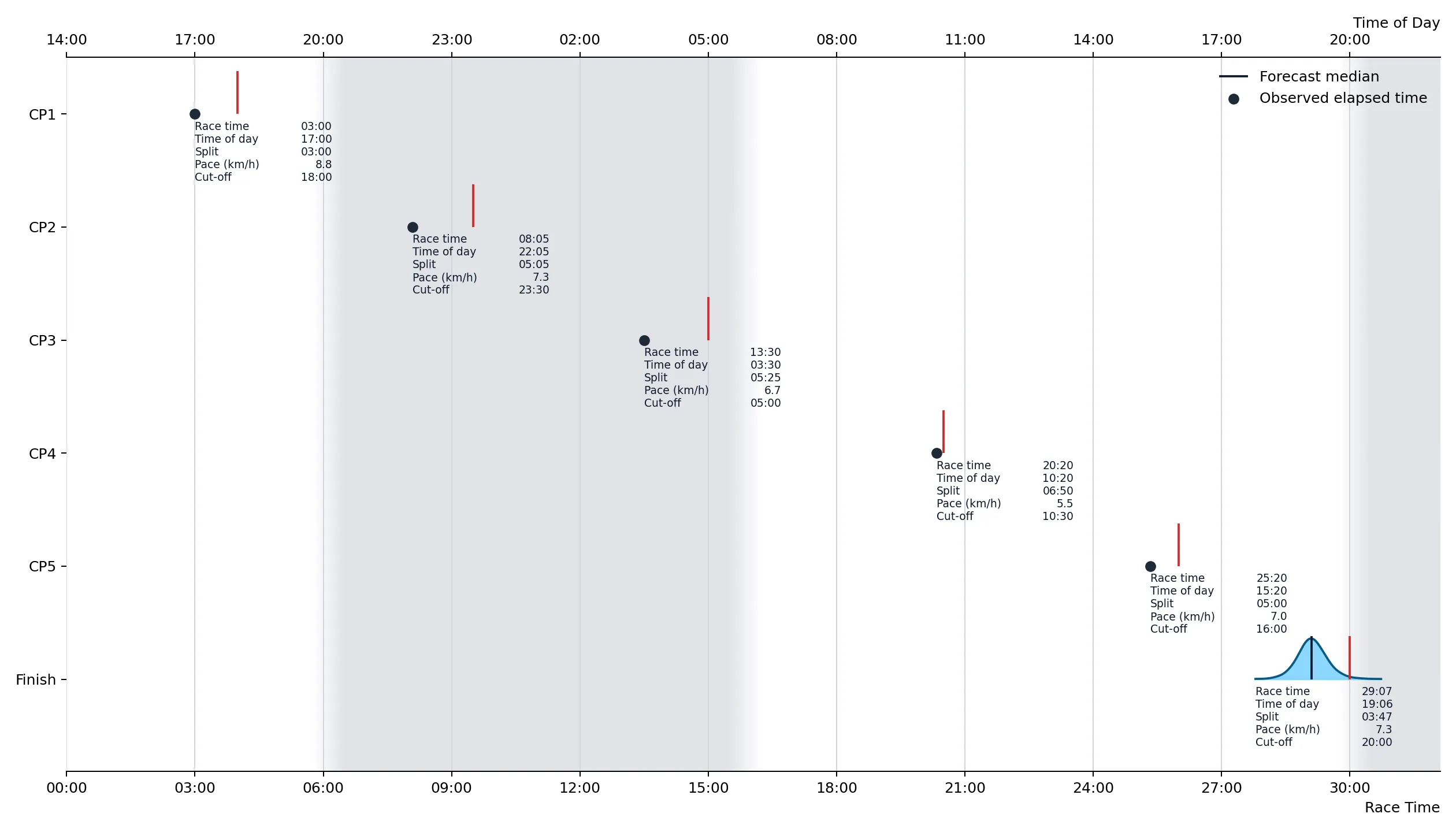
A strong push in the final leg would get them to the finish in just over 29 hours. That would be a gutsy effort given the misery of leg 4.
🚨 Caveat: The model can’t account for things going wrong.
Individual
Consider two individual entries: one (the rocket 🚀) has a blisteringly fast first leg (02:25) and the other (the tractor 🚜) gets off to a more sedate start (03:20). Let’s look at the rocket first.
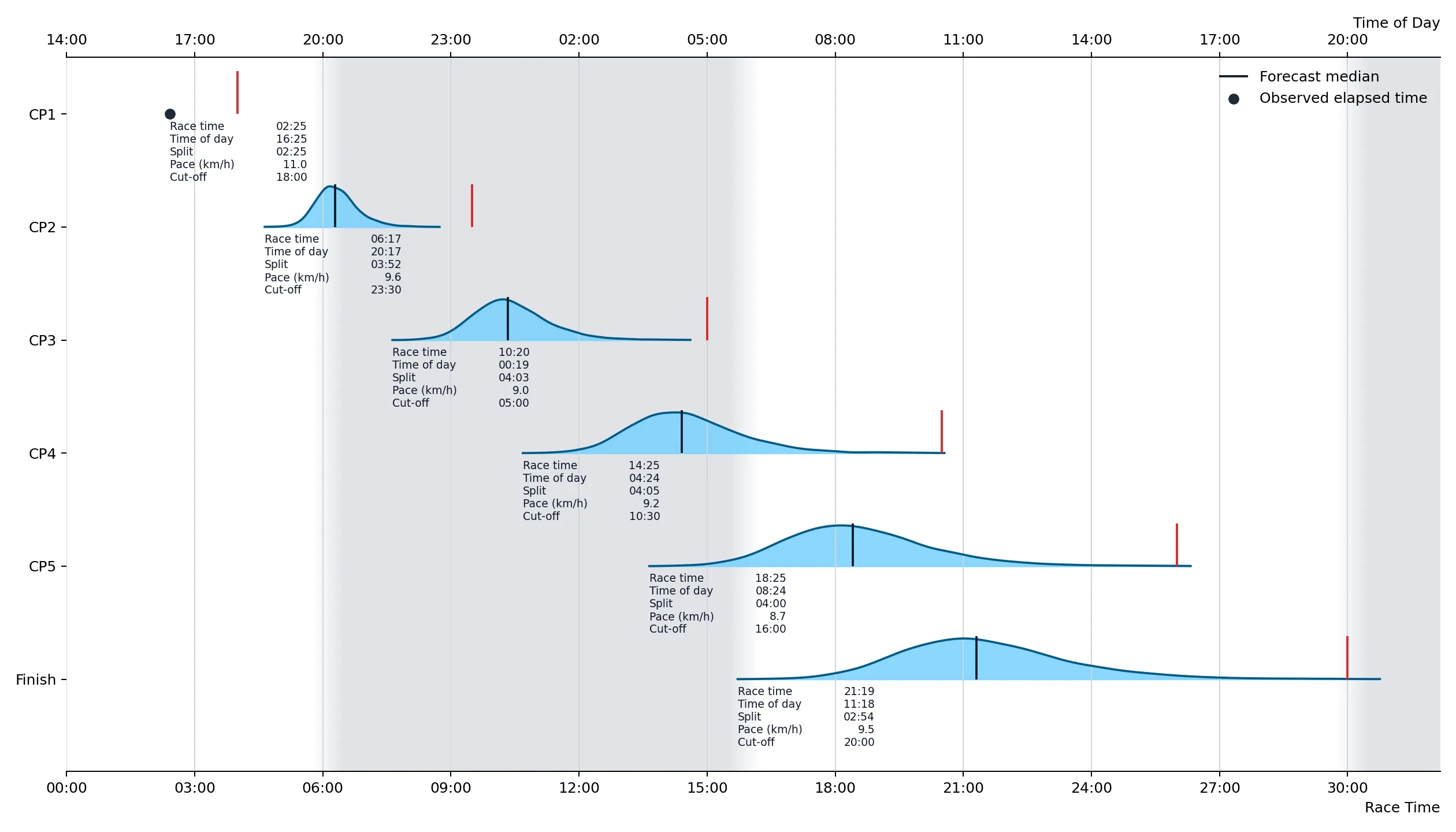
Based on the quick split for CP1, the model predicts comparably paced splits for the remaining legs, with an estimated finish time of 21:19. The median arrival times at the checkpoints are well within the corresponding cutoffs. The cutoff times for the last three legs do fall within the range of uncertainty predicted by the model, but they are so far down the tail that they realistically should not be a concern.
What about the tractor?
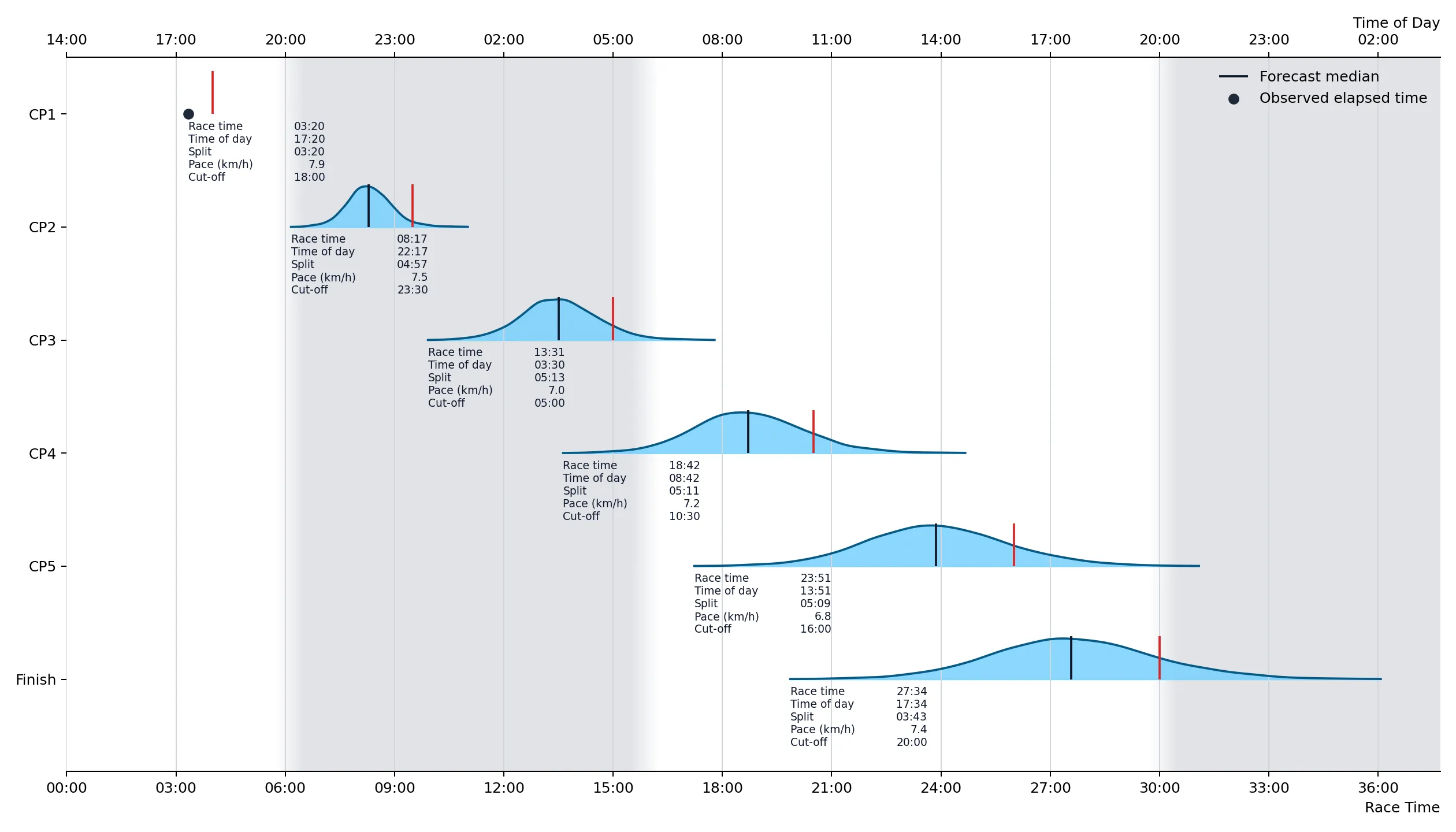
Because of his languid pace during the first leg, the predictions for subsequent legs are comparably unhurried, with a predicted finish time of 27:34. The cutoff times for later legs become progressively more of a concern.
But apparently he was just warming up. His pace increased for the second and third legs, changing the predicted finish time materially and making the cutoff times less of a concern. Because of the faster than expected pace over those two legs the predicted pace for the final three legs also increased.
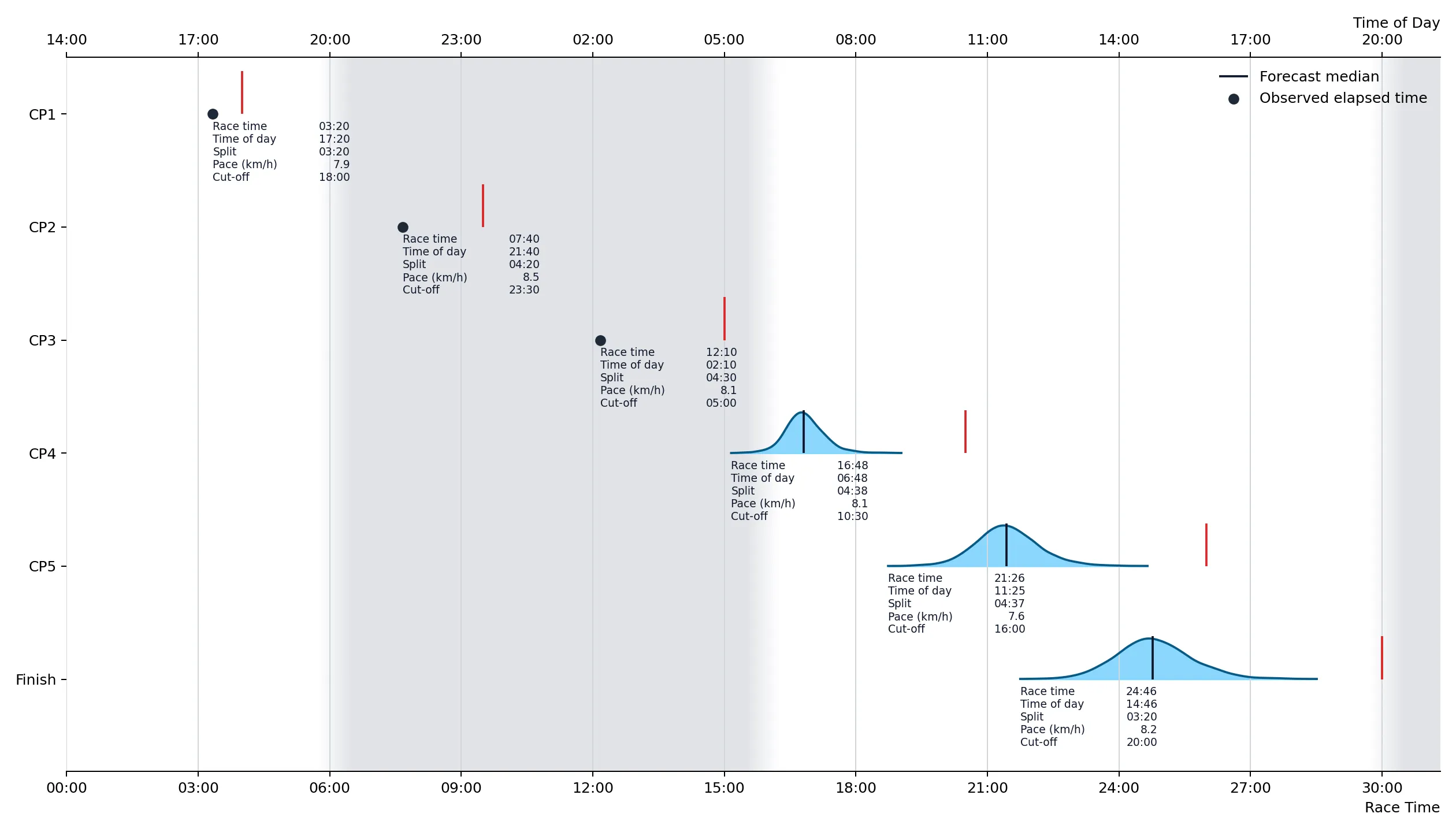
At CP4 he smashed a peanut butter flapjack and a double espresso, then finished the last two legs strong and ahead of the predicted finish time.
🚨 Caveat: The model can’t account for stimulants either.
Assumptions & Limits
Essentially, all models are wrong, but some are useful.
Predictions are only as good as the model’s assumptions and training data. The model may improve with additional data (we’ll have to wait until next year for that). Let’s be clear about the assumptions.
The model’s main assumptions are:
- the 2024, 2025 and 2026 results are comparable enough to pool despite different flow, weather, craft and crews;
- published checkpoint times are accurate;
- an entry will finish (retirement and cutoffs are not explicitly modelled), introducing selection bias;
- race category shifts the overall timing level, but doesn’t give each category a separate effect for each leg; and
- an entry’s pace is broadly shared across the race, rather than changing in a fully modelled way with fatigue, darkness or technical difficulties.
The model does not predict fatigue. It updates when later observations arrive. Fatigue should be reflected in progressively lower pace in later legs. The splits observed for those legs will inform the model of the effects of fatigue and they will then be factored into further predictions.
The model also doesn’t discriminate between possible causes of a bad leg (potentially fatigue, navigation challenges, mechanical failure or a toilet emergency). Whereas getting lost or having a broken rudder on one leg should not impact the subsequent legs, it’s reasonable to expect tired bodies to continue to get progressively more tired later in the race.
The uncertainty intervals include the historical sample, category, pace and leg variation. They do not forecast headwind, river flow, a broken seat, queues at a portage or a paddler having a bad night. They also do not include the probability of a DNF.
The model has no explicit year effect, route-distance term, portage count, craft type, paddler identity or start-group effect. The route is already partly represented because every historical entry paddled the same six legs. The other features need more data before they deserve their own coefficients. Adding them with limited data would turn the model into a machine for explaining noise.
What’s Next?
The model is based on the results for 92 finished entries in the Thames 200 Ultra during 2024, 2025 and 2026. The data covers a diverse range of capabilities across three categories and a limited sample of weather and flow conditions. It won’t tell you where a boat will be for every minute of the race (there’s live tracking for that!), but it does provide a reasonable estimate of checkpoint times. The estimate improves as observed checkpoint times are provided. Probably the most useful feature (IMHO) is that all predictions include an indication of uncertainty, and the uncertainty intervals contract as actual observations are added.
If there’s interest in the model, then I’ll continue to refine it and spin up an app ahead of the 2027 race. If not, it will have just been a fun exercise in Bayesian modelling.