A short while ago I was contracted to write a short piece entitled “Introduction to Fractals”. Admittedly it is hard to do justice to the topic in less than 1000 words.
Both of the illustrations were created with R. A copy of the original article can be found here.
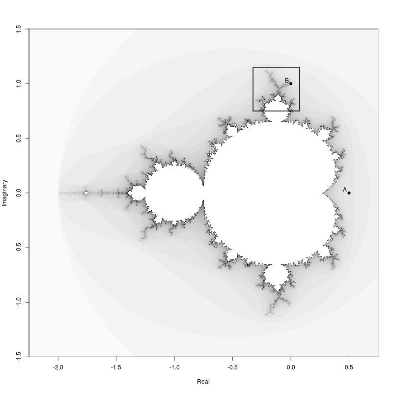
Mandelbrot Set
The Mandelbrot Set image was created using the Julia package.
library(Julia)
First an image of the entire set showing a region that we will zoom in on later.
npixel <- 2001
#
rshift <- -0.75
ishift <-  0.0
#
centre <- rshift + ishift * 1i
width <- 3.0
#
mandelbrot <- MandelImage(npixel, centre, width)

gray.colors <- gray((0:256)/ 256)

mandelbrot = t(mandelbrot[nrow(mandelbrot):1,])

x = 0:npixel / npixel * width - width / 2 + rshift
y = 0:npixel / npixel * width - width / 2 + ishift
#
image(x, y, mandelbrot, col = rev(gray.colors), useRaster = TRUE, xlab = "Real", ylab = "Imaginary",
      axes = FALSE)
box()
axis(1, at = seq(-2, 2, 0.5))
axis(2, at = seq(-2, 2, 0.5))
rect(-0.325, 0.75, 0.075, 1.15, border = "black", lwd = 2)
points(c(0.5, 0), c(0, 1), pch = 19)
text(c(0.5, 0), c(0, 1), labels = c("A", "B"), adj = c(1.55, -0.3))
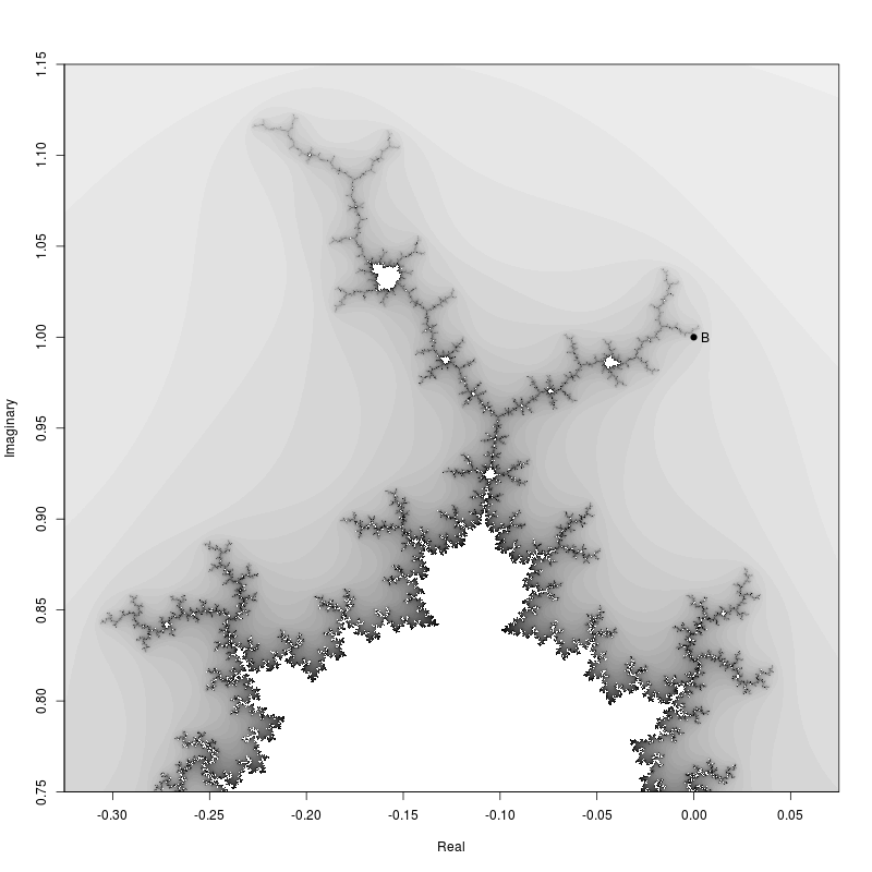
Then the zoomed in region.
npixel <- 2001;
#
rshift <- -0.125
ishift <-  0.95
#
centre <- rshift + ishift * 1i
width <- 0.4
#
zoom.mandelbrot <- MandelImage(npixel, centre, width)

zoom.mandelbrot = t(zoom.mandelbrot[nrow(zoom.mandelbrot):1,])

x = 0:npixel / npixel * width - width / 2 + rshift
y = 0:npixel / npixel * width - width / 2 + ishift
#
image(x, y, zoom.mandelbrot, col = rev(gray.colors), useRaster = TRUE, xlab = "Real",
      ylab = "Imaginary", axes = FALSE)
box()
axis(1, at = seq(-2, 2, 0.05))
axis(2, at = seq(-2, 2, 0.05))
points(c(0.5, 0), c(0, 1), pch = 19)
text(c(0.5, 0), c(0, 1), labels = c("A", "B"), adj = -0.75)
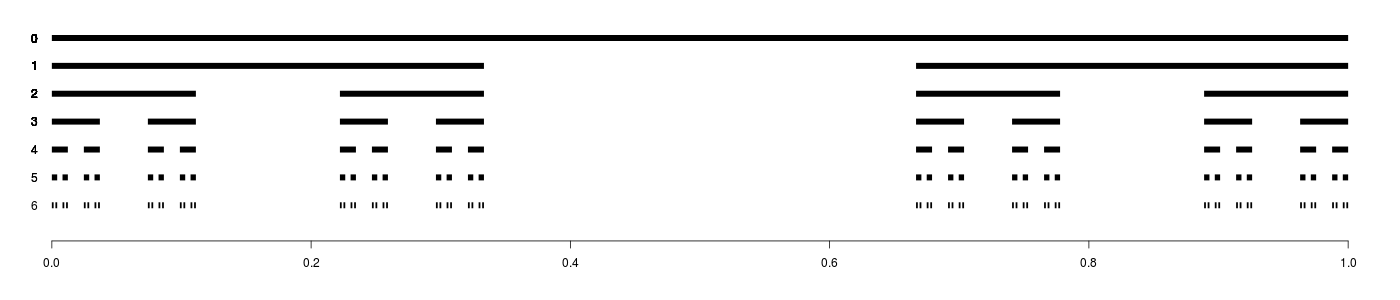
Cantor Set
The Cantor Set illustration was naturally created with a simple recursive algorithm.
cantor.set <- function(x) {
    y = list()
    for (n in x) {
        nL = n[1]
        nR = n[2]
        nl = nL + (nR - nL) / 3
        nr = nR - (nR - nL) / 3
        y[[length(y)+1]] <- c(nL, nl)
        y[[length(y)+1]] <- c(nr, nR)
    }
    return(y)
}

C = list()
#
C[[1]] = list(c(0, 1))
C[[2]] = cantor.set(C[[1]])
C[[3]] = cantor.set(C[[2]])
C[[4]] = cantor.set(C[[3]])
C[[5]] = cantor.set(C[[4]])
C[[6]] = cantor.set(C[[5]])
C[[7]] = cantor.set(C[[6]])
C[[8]] = cantor.set(C[[7]])
C[[9]] = cantor.set(C[[8]])
C[[10]] = cantor.set(C[[9]])

par(mar = c(4.1, 0.0, 2.1, 0.0))
plot(NULL, xlim = c(0,1), ylim = c(0, 7), axes = FALSE, xlab = "", ylab = "")
axis(1)
#
for (n in 1:7) {
    for (p in C[[n]]) {
        # print(p)
        lines(p, c(8-n ,8-n), lwd = 8, lend = "butt")
        text(x = 0, y = n, 7 - n, adj = c(3, 0.5))
    }
}