Percolation Threshold: Including Next-Nearest Neighbours

In my previous post about estimating the Percolation Threshold on a square lattice, I only considered flow from a given cell to its four nearest neighbours. It is a relatively simple matter to extend the recursive flow algorithm to include other configurations as well.

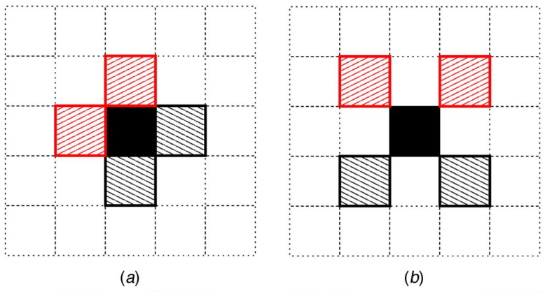
Malarz and Galam (2005) considered the problem of percolation on a square lattice for various ranges of neighbor links. Below is their illustration of (a) nearest neighbour “NN” and (b) next-nearest neighbour “NNN” links.

Implementing Next-Nearest Neighbours

There were at least two options for modifying the flow function to accommodate different configurations of neighbours: either they could be given as a function parameter or defined as a global variable. Although the first option is the best from an encapsulation perspective, it does make the recursive calls more laborious. I got lazy and went with the second option.

neighbours = c("NN")

flow <- function(g, i = NA, j = NA) {
   # -> Cycle through cells in top row
   #
   if (is.na(i) || is.na(j)) {
     for (j in 1:ncol(g)) {
       g = flow(g, 1, j)
     }
     return(g)
   }
   #
   # -> Check specific cell
   #
   if (i < 1 || i > nrow(g) || j < 1 || j > ncol(g)) return(g)
   #
   if (g[i,j] == OCCUPIED || g[i,j] == FLOW) return(g)
   #
   g[i,j] = FLOW
   
   if ("NN" %in% neighbours) {
     g = flow(g, i+1, j)           # down
     g = flow(g, i-1, j)           # up
     g = flow(g, i, j+1)           # right
     g = flow(g, i, j-1)           # left
   }
   if ("NNN" %in% neighbours) {
     g = flow(g, i+1, j+1)         # down+right
     g = flow(g, i-1, j+1)         # up+right
     g = flow(g, i+1, j-1)         # down+left
     g = flow(g, i-1, j-1)         # up+left
   }
   
   g
}

We will add a third example grid to illustrate the effect.

set.seed(1)
g1 = create.grid(12, 0.6)
g2 = create.grid(12, 0.4)
g3 = create.grid(12, 0.5)

Generating the compound plot with two different values of the global variable required a little thought. But fortunately the scoping rules in R allow for a rather nice implementation.

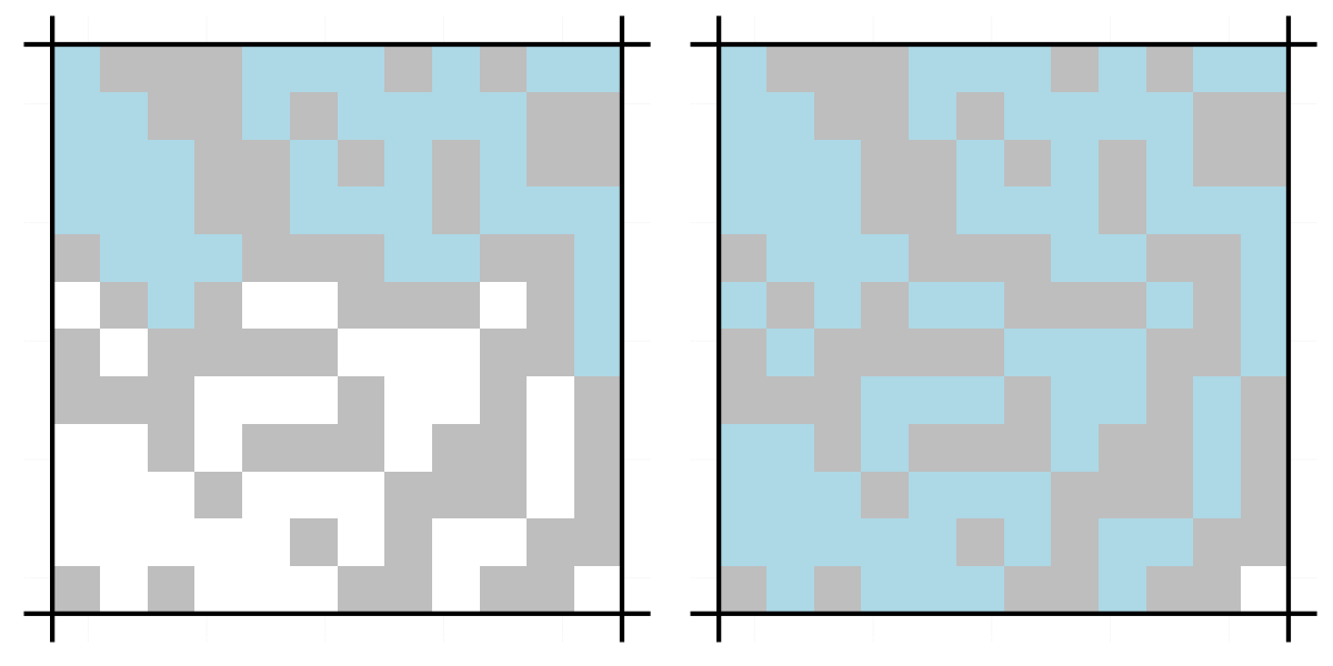
grid.arrange(
   {neighbours = c("NN"); visualise.grid(flow(g3))},
   {neighbours = c("NN", "NNN"); visualise.grid(flow(g3))},
   ncol = 2)

Here we have two plots for the same grid showing (left) NN and (right) NN+NNN percolation. Including the possibility of “diagonal” percolation extends the range of cells that are reachable and this grid, which does not percolate with just NN, does support percolation with NN+NNN.

No modifications are required to the percolation function.

neighbours = c("NN")

percolates(g1)

[1] FALSE

percolates(g2)

[1] TRUE

percolates(g3)

[1] FALSE

neighbours = c("NN", "NNN")

percolates(g1)

[1] FALSE

percolates(g2)

[1] TRUE

percolates(g3)

[1] TRUE

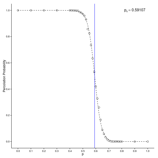
Effect on Percolation Threshold

Finally we can see the effect of including next-nearest neighbours on the percolation threshold. We perform the same logistic fit as previously.

(pcrit = - logistic.fit$coefficients[1] / logistic.fit$coefficients[2])

(Intercept) 
    0.59107 

1-pcrit

(Intercept) 
    0.40893

This agrees well with the result for NN+NNN from Table 1 in Malarz and Galam (2005).

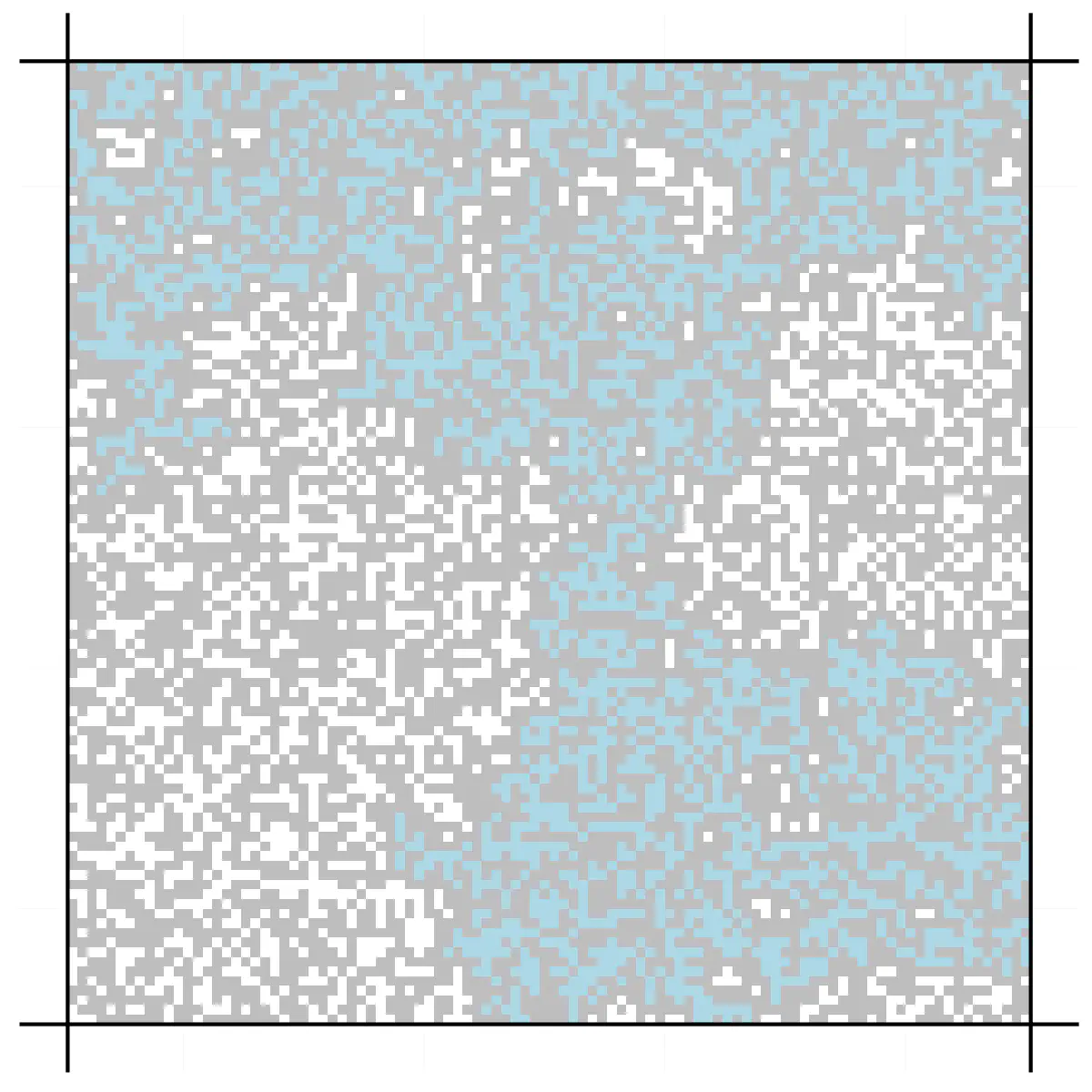
A Larger Lattice

Finally, let’s look at a larger lattice at the percolation threshold.

set.seed(1)

g4 = create.grid(100, pcrit)

percolates(g4)

[1] TRUE

References

• Malarz, K., & Galam, S. (2005). Square-lattice site percolation at increasing ranges of neighbor bonds. Physical Review E, 71(1), 016125. doi:10.1103/PhysRevE.71.016125.