In two previous posts in this series I have wrangled NEO orbital data into R and then solved Kepler’s Equation to get the eccentric anomaly for each NEO. The final stage in the visualisation of the NEO orbits will be the transformation of locations from the respective orbital planes into a single reference frame.
Reference Frame
The heliocentric ecliptic reference frame has the Sun at the origin and the ecliptic as the fundamental plane. For visualisation purposes we will be representing positions with respect to this plane in terms of rectangular (or Cartesian) coordinates.
Transformation
The transformation between the orbital plane \((X, Y, Z)\) and the heliocentric ecliptic coordinate system \((x, y, z)\) is achieved with
$$\begin{bmatrix}X\\\ Y\\\ Z\end{bmatrix} = \begin{bmatrix}\cos \phi_0 \cos \Omega - \sin \phi_0 \cos i \sin \Omega & \cos \phi_0 \sin \Omega + \sin \phi_0 \cos i \cos \Omega & \sin \phi_0 \sin i\\\ - \sin \phi_0 \cos \Omega - \cos \phi_0 \cos i \sin \Omega & - \sin \phi_0 \sin \Omega + \cos \phi_0 \cos i \cos \Omega & \cos \phi_0 \sin i\\\ \sin i \sin \Omega&- \sin i \cos \Omega&\cos i\end{bmatrix}\begin{bmatrix}x\\\ y\\\ z\end{bmatrix}$$
where \(\phi_0\) is the argument of perigee, \(i\) is the inclination and \(\Omega\) is the longitude of the ascending node.
Cartesian Coordinates
But, before we can use this transformation, we need to move to Cartesian Coordinates. This is easily accomplished.
orbits = within(orbits, {
  Z = 0
  Y = a * sqrt(1 - e**2) * sin(E)
  X = a * cos(E) - a * e
})
head(orbits)
             Object Epoch      a       e        i       w   Node       M     q.    Q    P    H     MOID class hazard       E  theta        X        Y Z
1  100004 (1983 VA) 56800 2.5959 0.69970 0.284254 0.21050 1.3498 1.40950 0.7795 4.41 4.18 16.4 0.176375   APO  FALSE 2.03512 2.6336 -2.97885  1.65824 0
2 100085 (1992 UY4) 56800 2.6398 0.62481 0.048926 0.66896 5.3826 0.22042 0.9904 4.29 4.29 17.8 0.015111   APO   TRUE 0.54358 1.0511  0.60993  1.06602 0
3 100756 (1998 FM5) 56800 2.2686 0.55202 0.201156 5.43895 3.0869 4.82500 1.0163 3.52 3.42 16.1 0.100211   APO  FALSE 4.31582 3.8282 -2.12857 -1.74482 0
4  100926 (1998 MQ) 56800 1.7827 0.40777 0.422864 2.42053 3.8599 3.42868 1.0558 2.51 2.38 16.7 0.128731   AMO  FALSE 3.34594 3.2744 -2.47255 -0.33031 0
5  101869 (1999 MM) 56800 1.6243 0.61071 0.083167 4.68848 1.9388 0.75843 0.6323 2.62 2.07 19.3 0.001741   APO   TRUE 1.35497 2.0445 -0.64413  1.25637 0
6 101873 (1999 NC5) 56800 2.0295 0.39332 0.798850 5.15317 2.2489 5.65453 1.2312 2.83 2.89 16.3 0.437678   AMO  FALSE 5.33502 4.9613  0.38531 -1.51575 0
Note that the \(Z\) component is zero for all of the orbits since this is the coordinate which is perpendicular to the orbital planes (and all of the orbits lie strictly within the fundamental plane of their respective coordinate systems).
Now we need to generate a transformation matrix for each orbit. We will wrap that up in a function.
transformation.matrix <- function(w, Node, i) {
  a11 =   cos(w) * cos(Node) - sin(w) * cos(i) * sin(Node)
  a12 =   cos(w) * sin(Node) + sin(w) * cos(i) * cos(Node)
  a13 =   sin(w) * sin(i)

  a21 = - sin(w) * cos(Node) - cos(w) * cos(i) * sin(Node)
  a22 = - sin(w) * sin(Node) + cos(w) * cos(i) * cos(Node)
  a23 =   cos(w) * sin(i)

  a31 =   sin(i) * sin(Node)
  a32 = - sin(i) * cos(Node)
  a33 =   cos(i)

  matrix(c(a11, a12, a13, a21, a22, a23, a31, a32, a33), nrow = 3, byrow = TRUE)
}
First we will try this out for a single object.
(A = do.call(transformation.matrix, orbits[1, c("w", "Node", "i")]))
          [,1]       [,2]     [,3]
[1,]  0.018683  0.9981068 0.058599
[2,] -0.961656  0.0018992 0.274251
[3,]  0.273620 -0.0614756 0.959871
# We want to invert this transformation, so we need to invert the matrix. However, since this is a
# rotation matrix, the inverse and the transpose are the same... (we will use this fact later!)
#
A = solve(A)
#
A %*% matrix(unlist(orbits[1, c("X", "Y", "Z")]), ncol = 1)
         [,1]
[1,] -1.65031
[2,] -2.97006
[3,]  0.28022
That looks pretty reasonable. Now we need to do that systematically to all of the objects.
require(plyr)

orbits = ddply(orbits, .(Object), function(df) {
  A = transformation.matrix(df$w, df$Node, df$i)
  #
  # Invert transformation matrix
  #
  A = t(A)
  #
  # Transform to reference frame
  #
  r = A %*% matrix(unlist(df[, c("X", "Y", "Z")]), ncol = 1)
  #
  r = matrix(r, nrow = 1)
  colnames(r) = c("x", "y", "z")
  #
  cbind(df, r)
})
head(orbits)
             Object Epoch      a       e        i       w   Node       M     q.    Q    P    H     MOID class hazard       E  theta        X        Y Z        x        y         z
1  100004 (1983 VA) 56800 2.5959 0.69970 0.284254 0.21050 1.3498 1.40950 0.7795 4.41 4.18 16.4 0.176375   APO  FALSE 2.03512 2.6336 -2.97885  1.65824 0 -1.65031 -2.97006  0.280216
2 100085 (1992 UY4) 56800 2.6398 0.62481 0.048926 0.66896 5.3826 0.22042 0.9904 4.29 4.29 17.8 0.015111   APO   TRUE 0.54358 1.0511  0.60993  1.06602 0  0.83726  0.89659  0.059398
3 100756 (1998 FM5) 56800 2.2686 0.55202 0.201156 5.43895 3.0869 4.82500 1.0163 3.52 3.42 16.1 0.100211   APO  FALSE 4.31582 3.8282 -2.12857 -1.74482 0  2.69099 -0.57127  0.086300
4  100926 (1998 MQ) 56800 1.7827 0.40777 0.422864 2.42053 3.8599 3.42868 1.0558 2.51 2.38 16.7 0.128731   AMO  FALSE 3.34594 3.2744 -2.47255 -0.33031 0 -2.39321 -0.41532 -0.568055
5  101869 (1999 MM) 56800 1.6243 0.61071 0.083167 4.68848 1.9388 0.75843 0.6323 2.62 2.07 19.3 0.001741   APO   TRUE 1.35497 2.0445 -0.64413  1.25637 0 -1.02820  0.96622  0.050998
6 101873 (1999 NC5) 56800 2.0295 0.39332 0.798850 5.15317 2.2489 5.65453 1.2312 2.83 2.89 16.3 0.437678   AMO  FALSE 5.33502 4.9613  0.38531 -1.51575 0  1.29744 -0.50408 -0.713095
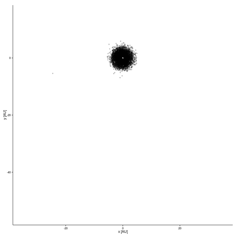
Looks good. Time to generate some plots. First we will look at the distribution of objects in the solar-ecliptic plane. Most of them are clustered within a few AU of the Sun, but there are a few stragglers at much larger distances.
library(ggplot2)

ggplot(orbits, aes(x = x, y = y)) +
  geom_point(alpha = 0.25) +
  xlab("x [AU]") + ylab("y [AU]") +
  scale_x_continuous(limits = c(-35, 35)) + scale_y_continuous(limits = c(-55, 15)) +
  theme_classic() +
  theme(aspect.ratio = 1)
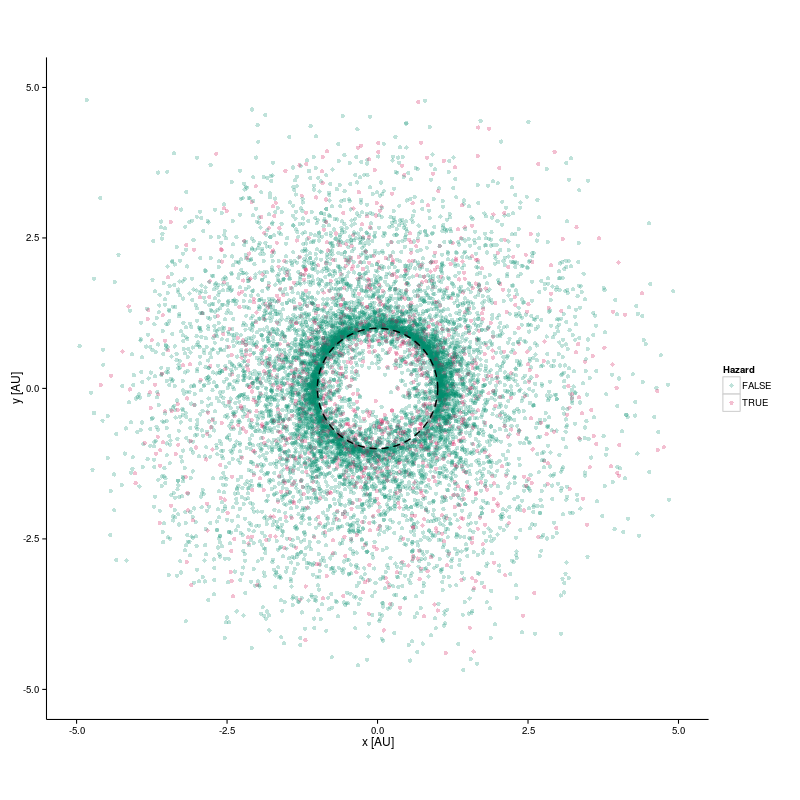
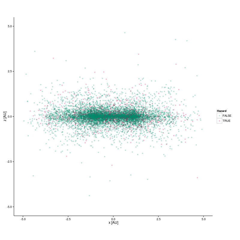
We can zoom in on the central region within 5 AU of the Sun. We will also produce a projection onto the $$ x-z $$ plane so that we can see how far these objects lie above or below the ecliptic plane.
library(grid)

ggplot(orbits, aes(x = x, y = y)) +
  geom_point(aes(colour = hazard), alpha = 0.25) +
  scale_colour_discrete("Hazard", h = c(180, 0), c = 150, l = 40) +
  xlab("x [AU]") + ylab("y [AU]") +
  scale_x_continuous(limits = c(-5, 5)) + scale_y_continuous(limits = c(-5, 5)) +
  annotation_custom(grob = circleGrob(
    r = unit(0.5, "npc"), gp = gpar(fill = "transparent", col = "black", lwd = 2, lty = "dashed")),
    xmin=-1, xmax=1, ymin=-1, ymax=1) +
  theme_classic() +
  theme(aspect.ratio = 1)

ggplot(orbits, aes(x = x, y = z)) +
  geom_point(aes(colour = hazard), alpha = 0.25) +
  scale_colour_discrete("Hazard", h = c(180, 0), c = 150, l = 40) +
  xlab("x [AU]") + ylab("z [AU]") +
  scale_x_continuous(limits = c(-5, 5)) + scale_y_continuous(limits = c(-5, 5)) +
  theme_classic() +
  theme(aspect.ratio = 1)
The dashed circle indicates the orbit of the Earth. Most of the objects are clustered around this orbit.
Although there are numerous objects which lie a few AU on either side of the ecliptic plane, the vast majority are (like the planets) very close to or on the plane itself.
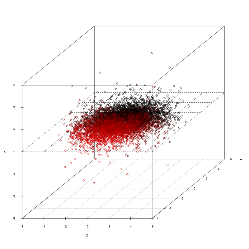
Finally a three dimensional visualisation. I would have liked to rotate this plot to try and get a better perspective, but I could not manage that with scatterplot3d. It’s probably not the right tool for that particular job.
library(scatterplot3d)

orbits.3d <- with(orbits, scatterplot3d(x, y, z, xlim = c(-5, 5), ylim = c(-5, 5), highlight.3d = TRUE))
orbits.3d$plane3d(c(0, 0, 0))
I have enjoyed working with these data. My original plan was to leave the project at this point. But, since the data are neatly classified according to two different schemes, it presents a good opportunity to try out some classification models. More on that shortly.