{hagr} Linnaean Classification

I’ve taken another look at the {hagr} data, which I wrote about previously. This time I’m focusing on the hierarchy of creatures.

Taxonomic Rank

The Linnaean Taxonomy is a hierarchical classification system for organisms devised by Carl Linnaeus. An organism is assigned to the following levels in the hierarchy (in increasing order or granularity):

domain
kingdom
phylum
class
order
family
genus and
species.

The relative level of a group of organisms in this hierarchy determines its taxonomic rank.

💡 The Linnaean Taxonomy was developed way before the idea of evolution arose. As a consequence, despite being a useful framework for classifying organisms, it does not take into account evolutionary relationships.

Taxonomic ranks. Image from [Wikipedia](https://en.wikipedia.org/wiki/Taxonomic_rank).

Let’s take a look at the classification data in the {hagr} package.

library(hagr)

Linnaean Taxonomic Levels

We’ll start at the top level, domain.

age %>% count(domain, sort = TRUE)

# A tibble: 1 × 2
  domain      n
  <chr>   <int>
1 Eukarya  4219

There’s only one domain, Eukarya, present. We don’t have any information on Bacteria or Archaea (single-celled organisms).

If we dig down one level then we find that the Eukarya domain consists of three kingdoms: Animalia, Fungi and Plantae. There’s actually a fourth kingdom in Eukarya, Protista, however there’s no data for it in age.

age %>% count(kingdom, sort = TRUE)

# A tibble: 3 × 2
  kingdom      n
  <fct>    <int>
1 Animalia  4215
2 Fungi        3
3 Plantae      1

It’s clear that Animalia is the dominant kingdom, so let’s focus on that exclusively.

animalia <- age %>% filter(kingdom == "Animalia")

The next level in the hierarchy is phylum.

animalia %>% count(phylum, sort = TRUE)

# A tibble: 7 × 2
  phylum            n
  <fct>         <int>
1 Chordata       4200
2 Arthropoda        8
3 Echinodermata     2
4 Porifera          2
5 Cnidaria          1
6 Mollusca          1
7 Nematoda          1

It appears that Chordata is the dominant phylum in the data, so let’s further narrow our attention.

chordata <- animalia %>% filter(phylum == "Chordata")

Now let’s drill all the way down to genus.

chordata %>% count(class, order, family, genus, sort = TRUE)

# A tibble: 2,035 × 5
   class          order             family           genus            n
   <fct>          <fct>             <fct>            <fct>        <int>
 1 Teleostei      Scorpaeniformes   Scorpaenidae     Sebastes        49
 2 Teleostei      Perciformes       Percidae         Etheostoma      35
 3 Aves           Passeriformes     Parulidae        Setophaga       23
 4 Teleostei      Cypriniformes     Cyprinidae       Notropis        23
 5 Mammalia       Chiroptera        Vespertilionidae Myotis          21
 6 Reptilia       Squamata          Viperidae        Crotalus        19
 7 Teleostei      Perciformes       Lutjanidae       Lutjanus        18
 8 Aves           Psittaciformes    Psittacidae      Amazona         17
 9 Chondrichthyes Carcharhiniformes Carcharhinidae   Carcharhinus    17
10 Aves           Falconiformes     Falconidae       Falco           15
# … with 2,025 more rows

Adding in species takes you to the most granular level in the hierarchy.

chordata %>% select(class, order, family, genus, species, common_name)

# A tibble: 4,200 × 6
   class    order family         genus    species    common_name            
   <fct>    <fct> <fct>          <fct>    <fct>      <chr>                  
 1 Amphibia Anura Bombinatoridae Bombina  bombina    Firebelly toad         
 2 Amphibia Anura Bombinatoridae Bombina  orientalis Oriental firebelly toad
 3 Amphibia Anura Bombinatoridae Bombina  variegata  Yellow-bellied toad    
 4 Amphibia Anura Bufonidae      Anaxyrus americanus American toad          
 5 Amphibia Anura Bufonidae      Anaxyrus boreas     Western toad           
 6 Amphibia Anura Bufonidae      Anaxyrus canorus    Yosemite toad          
 7 Amphibia Anura Bufonidae      Anaxyrus cognatus   Great plains toad      
 8 Amphibia Anura Bufonidae      Anaxyrus debilis    Green toad             
 9 Amphibia Anura Bufonidae      Anaxyrus hemiophrys Canadian toad          
10 Amphibia Anura Bufonidae      Anaxyrus punctatus  Red-spotted toad       
# … with 4,190 more rows

💡 The combination of genus and species gives the binomial scientific name for organisms. For example, the Killer Whale is Orcinus orca.

age %>%
  filter(str_detect(common_name, "^(Killer|Blue|Sperm) whale$")) %>%
  select(class:common_name)

# A tibble: 3 × 6
  class    order   family          genus        species       common_name 
  <fct>    <fct>   <fct>           <fct>        <fct>         <chr>       
1 Mammalia Cetacea Balaenopteridae Balaenoptera musculus      Blue whale  
2 Mammalia Cetacea Delphinidae     Orcinus      orca          Killer whale
3 Mammalia Cetacea Physeteridae    Physeter     macrocephalus Sperm whale

Growing a Tree

We’ll use {ggtree} to construct a phylogenetic tree from domain down to order.

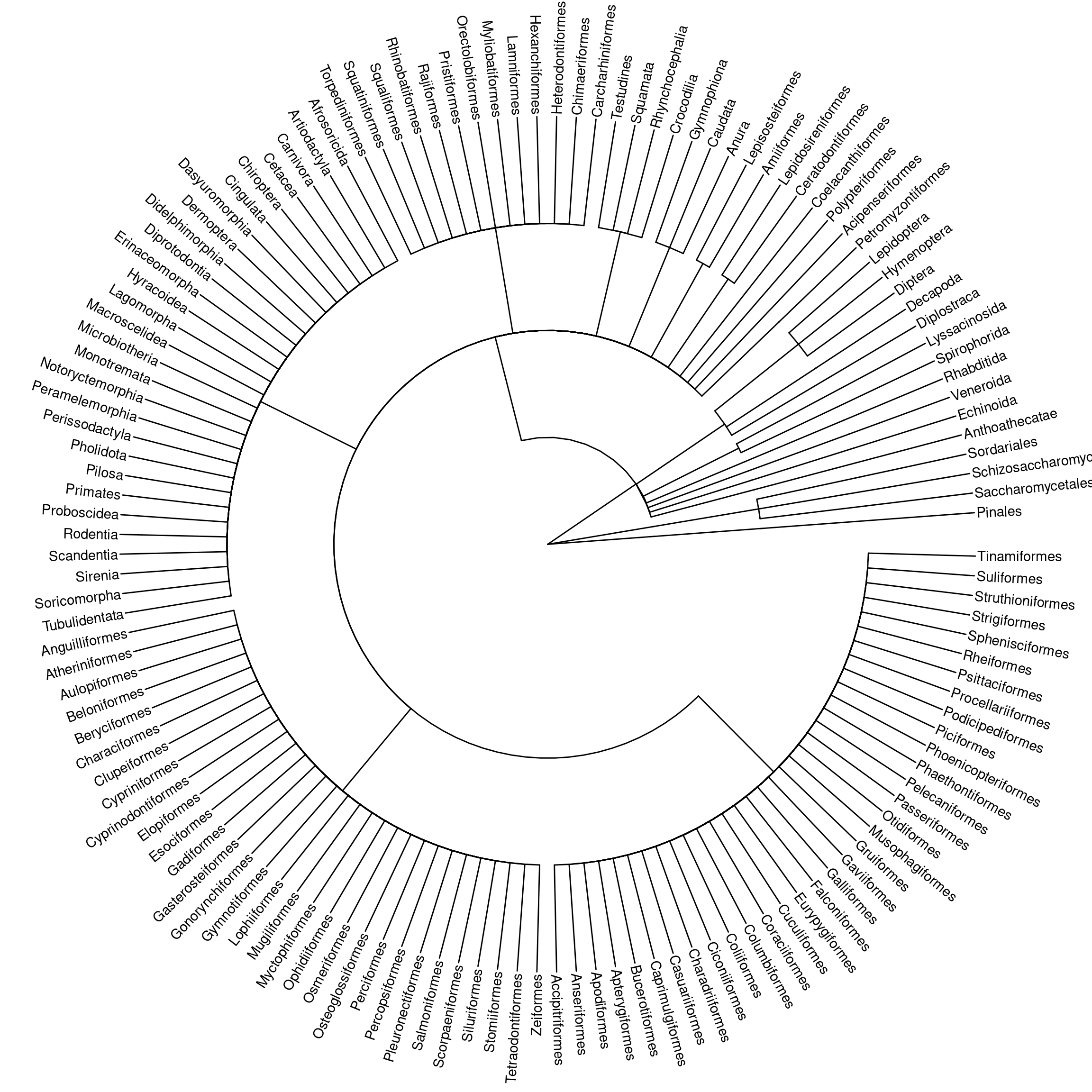
The dominance of the Chordata phylum in the data is readily apparent! It’d be nice to include more levels in this tree, but it gets very big and rather messy.

There’s such a wealth of cool information in this dataset. Really indebted to the Human Ageing Genomic Resources project for putting it together and generously sharing it.