I’m going to be writing a series of posts which will look at some applications of R (and perhaps Python) to financial modelling. We’ll start here by pulling some stock data into R, calculating the daily returns and then looking at correlations and simple volatility estimates.
Data
I was looking for a chunky set of stock data, preferably something that was available at higher than daily time resolution. The data from Kaggle for NIFTY 100 stocks on the Indian Stock Market seemed a decent fit.
📌 Although I wanted intraday data I won’t be using it for the moment and will start by aggregating the data up to daily resolution.
List of Data Frames
Data for each of the stocks is in a separate CSV file. Start by iterating over these using map_dfr() and loading them into a single data frame.
FILES <- list.files("data", pattern=".csv$", full.names = TRUE)

load <- function(path) {
  read_csv(path, show_col_types = FALSE) %>%
    mutate(
      symbol = sub(".csv$", "", basename(path)),
      time = as.POSIXct(date),
      date = as.Date(time)
    ) %>%
    group_by(symbol, date) %>%
    arrange(time) %>%
    # Summarise the daily closing price.
    summarise(
      close = last(close),
      .groups = "drop"
    )
}

stocks <- map_dfr(FILES, load)
How many records do we have and what does the data look like?
nrow(stocks)[1] 151932head(stocks)# A tibble: 6 × 3
symbol date close
<chr> <date> <dbl>
1 ACC 2015-02-02 1515.
2 ACC 2015-02-03 1512.
3 ACC 2015-02-04 1490
4 ACC 2015-02-05 1500.
5 ACC 2015-02-06 1513.
6 ACC 2015-02-09 1504.We could work with them en masse, but it’s going to be easier to split into a list of data frames, one for each stock.
stocks <- split(stocks, stocks$symbol)
length(stocks)
[1] 87names(stocks) [1] "ACC" "ADANIENT" "ADANIPORTS" "AMBUJACEM" "APOLLOHOSP" "ASIANPAINT" "AUROPHARMA" "AXISBANK" "BAJAJ-AUTO" "BAJAJFINSV" "BAJFINANCE" "BANKBARODA"
[13] "BERGEPAINT" "BHARTIARTL" "BIOCON" "BOSCHLTD" "BPCL" "BRITANNIA" "CADILAHC" "CHOLAFIN" "CIPLA" "COALINDIA" "COLPAL" "DABUR"
[25] "DIVISLAB" "DLF" "DRREDDY" "EICHERMOT" "GAIL" "GODREJCP" "GRASIM" "HAVELLS" "HCLTECH" "HDFC" "HDFCBANK" "HEROMOTOCO"
[37] "HINDALCO" "HINDPETRO" "HINDUNILVR" "ICICIBANK" "IGL" "INDUSINDBK" "INDUSTOWER" "INFY" "IOC" "ITC" "JINDALSTEL" "JSWSTEEL"
[49] "JUBLFOOD" "KOTAKBANK" "LT" "LUPIN" "M_M" "MARICO" "MARUTI" "MCDOWELL-N" "MUTHOOTFIN" "NAUKRI" "NESTLEIND" "NIFTY50"
[61] "NIFTYBANK" "NMDC" "NTPC" "ONGC" "PEL" "PIDILITIND" "PIIND" "PNB" "POWERGRID" "RELIANCE" "SAIL" "SBIN"
[73] "SHREECEM" "SIEMENS" "SUNPHARMA" "TATACONSUM" "TATAMOTORS" "TATASTEEL" "TCS" "TECHM" "TITAN" "TORNTPHARM" "ULTRACEMCO" "UPL"
[85] "VEDL" "WIPRO" "YESBANK" There are 87 distinct stocks and a number of names there that you might recognise.
Time Series
Now convert them into individual xts objects and concatenate to form a single xts object with the closing time series for each of the stocks.
stocks <- stocks %>%
  map(~{
    ts <- xts(x = .[["close"]], order.by = .[["date"]])
    colnames(ts) <- unique(.$symbol)

    ts
  })

stocks <- do.call(merge, stocks) %>% na.omit()
stocks <- stocks["2016-01-01/2022-01-01"]
We now have a multivariate time series. How many individual series and how many observations?
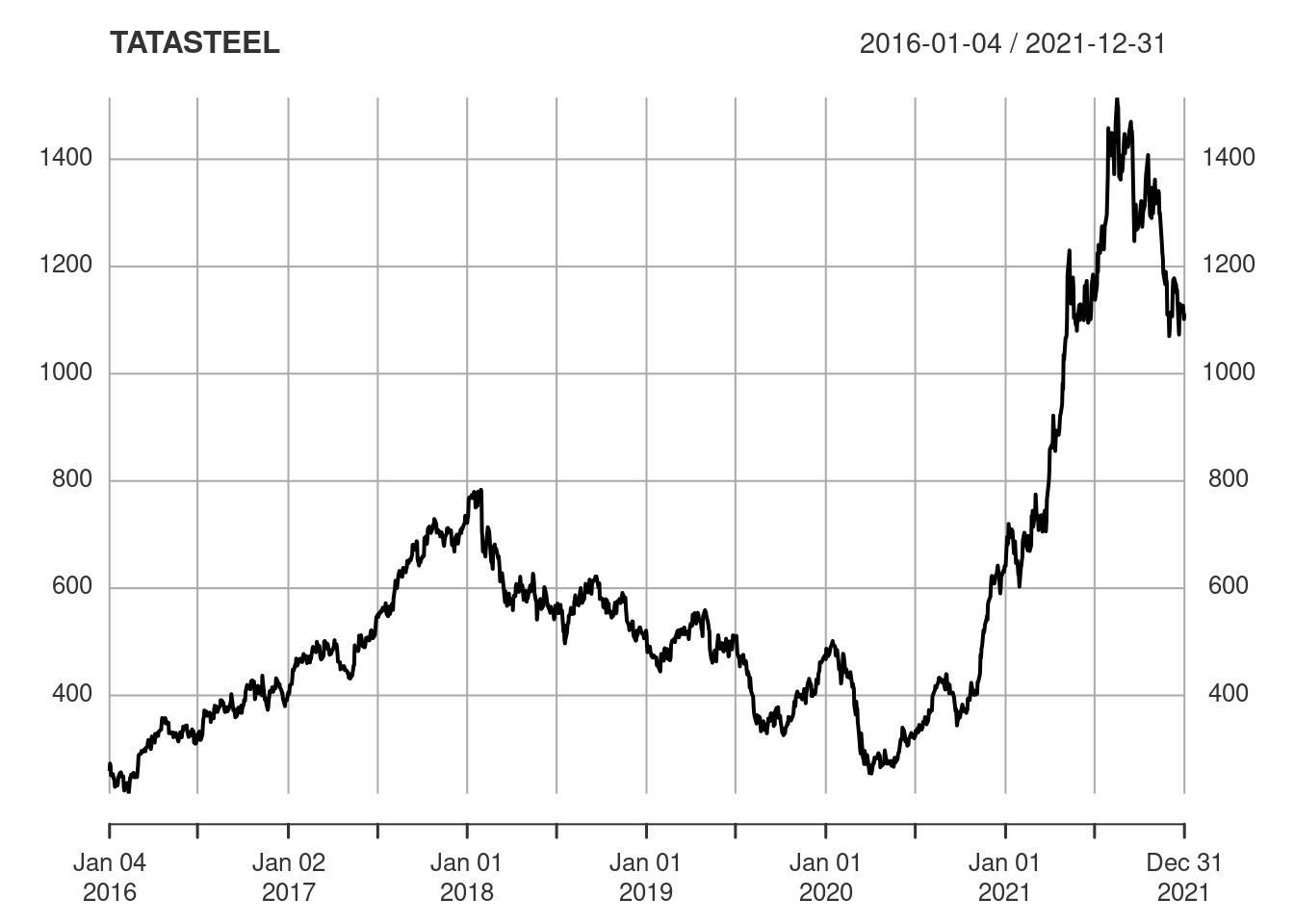
dim(stocks)[1] 1485 87That’s 87 time series and 1485 observations for each of them. Each time series looks like this:
head(stocks$TATASTEEL) TATASTEEL
2016-01-04 259.00
2016-01-05 272.95
2016-01-06 268.75
2016-01-07 251.00
2016-01-08 254.55
2016-01-11 252.90We can print the closing prices but it’s more useful to have a plot.
Returns
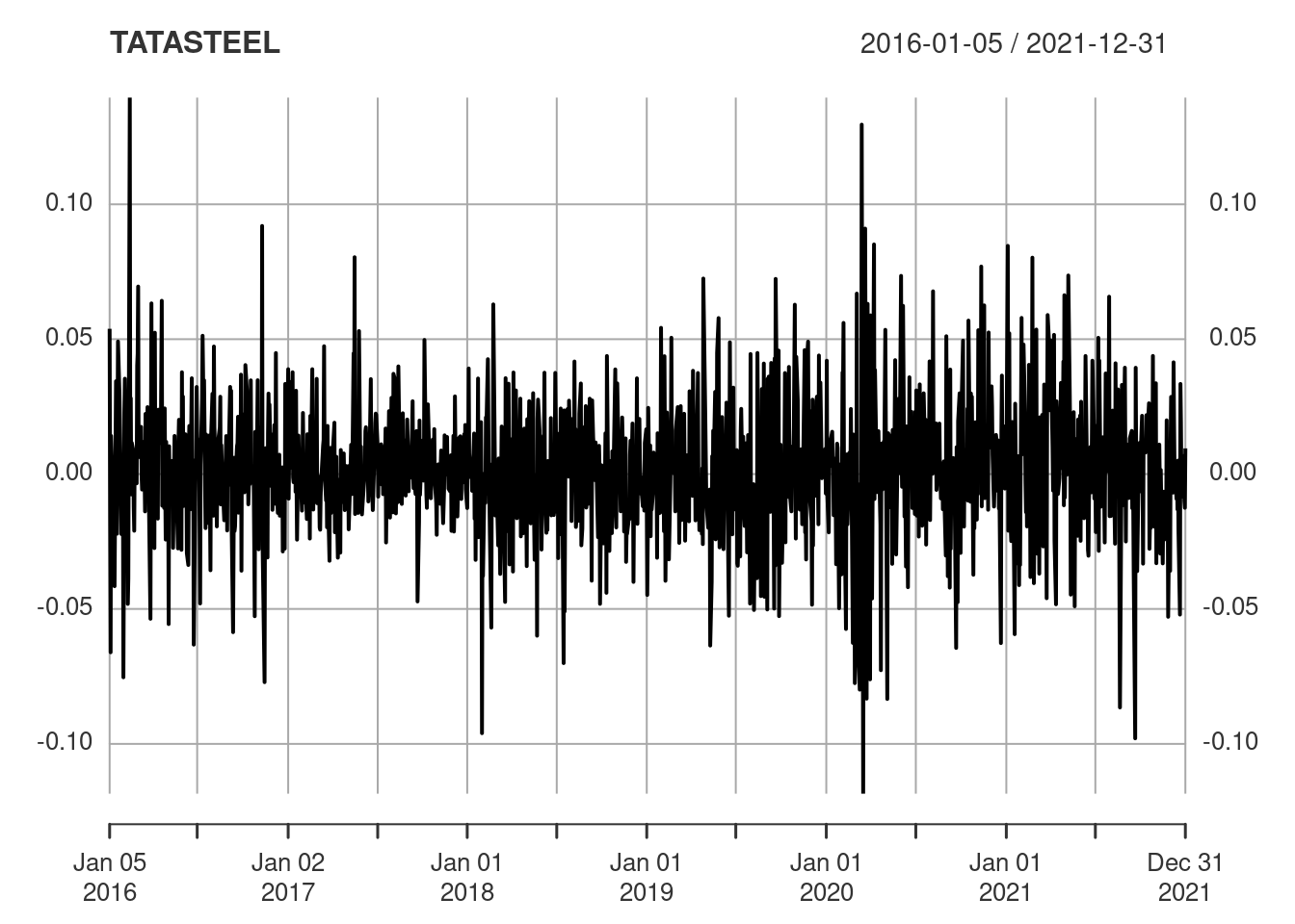
For analytical purposes the absolute daily closing price is not as interesting as the daily return, which can be easily calculated but we’ll use CalculateReturns() from {PerformanceAnalytics} for convenience.
returns <- CalculateReturns(stocks) %>% na.omit()Plot the corresponding return time series.
Stationarity
We are going to be building time series models for the returns, so it would be prudent to check whether the time series data are stationary.
library(tseries)

adf.test(TATASTEEL, alternative = "stationary")
    Augmented Dickey-Fuller Test

data:  TATASTEEL
Dickey-Fuller = -10.003, Lag order = 11, p-value = 0.01
alternative hypothesis: stationary
For the Augmented Dickey-Fuller (ADF) test the null hypothesis is non-stationarity. Since the outcome of the test is significant we can reject this hypothesis and state that the series is indeed stationary.
library(urca)

ur.kpss(TATASTEEL)
#######################################
# KPSS Unit Root / Cointegration Test #
#######################################

The value of the test statistic is: 0.2072
In contrast to the ADF test, the Kwiatkowski-Phillips-Schmidt-Shin (KPSS) test has stationarity as the null hypothesis. Since the result of the test is insignificant we should not contemplate rejected this hypothesis.
The results of both tests suggest that the returns time series is stationary.
Variability & Volatility
There’s a lot of diversity in the return time series across the collection of stocks. To illustrate, here are the series for a collection of them.
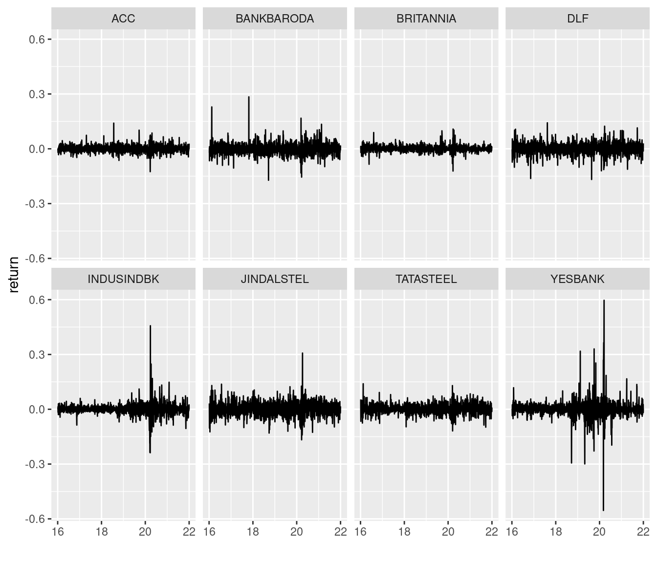
ACC has a roughly consistent low level of return variability over the six years. By contrast, Yes Bank has periods of increased variability starting in the latter part of 2018.
Daily Volatility
It would be useful if we had a number (or numbers) to describe the relative level of variability. Volatility is a statistical measure of the dispersion of returns and is calculated as either the standard deviation or variance of the returns. In general, the higher the volatility, the riskier the security.
# Pull out the returns for two specific stocks.
#
ACC <- returns$ACC
YESBANK <- returns$YESBANK
Let’s start by calculating the standard deviations of those stocks over the entire data period.
# Daily volatility.
#
sd(ACC)
[1] 0.0184169sd(YESBANK)[1] 0.04682746As expected the volatility of Yes Bank is higher than that of ACC.
Annualised Volatility
These values can be thought of as the average daily variation in the stock’s return. However, what’s more commonly used is the annualised value, which takes into account the fact that there are on average 252 trading days in each year and reflects the average variation in the stock’s return over the course of a year.
# Annualised volatility.
#
sqrt(252) * sd(ACC)
[1] 0.2923593sqrt(252) * sd(YESBANK)[1] 0.7433629Varying Volatility
It’s instructive to look at the volatility for shorter periods of time. Let’s compare the volatility of those two stocks in 2017 and 2020.
sqrt(252) * sd(ACC["2017"])[1] 0.2344968sqrt(252) * sd(YESBANK["2017"])[1] 0.2665718In 2017 the volatilities of ACC and Yes Bank are comparable.
sqrt(252) * sd(ACC["2020"])[1] 0.3900236sqrt(252) * sd(YESBANK["2020"])[1] 1.283764However, in 2020 Yes Bank is substantially more volatile than ACC.
Of course you can make these volatility calculations progressively more granular. However, as time intervals get shorter you have less data, so each of the individual measurements becomes less reliable. We’ll be modelling the time variation of volatility in upcoming posts.
Outliers
The returns might include significant outliers that would likely bias any derived results. We can use winsorisation to reduce the effect of extreme outliers in the data. The Return.clean() function from {PerformanceAnalytics} can be used to apply clean.boudt() to the data.
yesbank <- Return.clean(YESBANK, method = "boudt")In the plot below the raw data are in black and the cleaned data are in blue. The extrema are reduced in magnitude in the cleaned data.
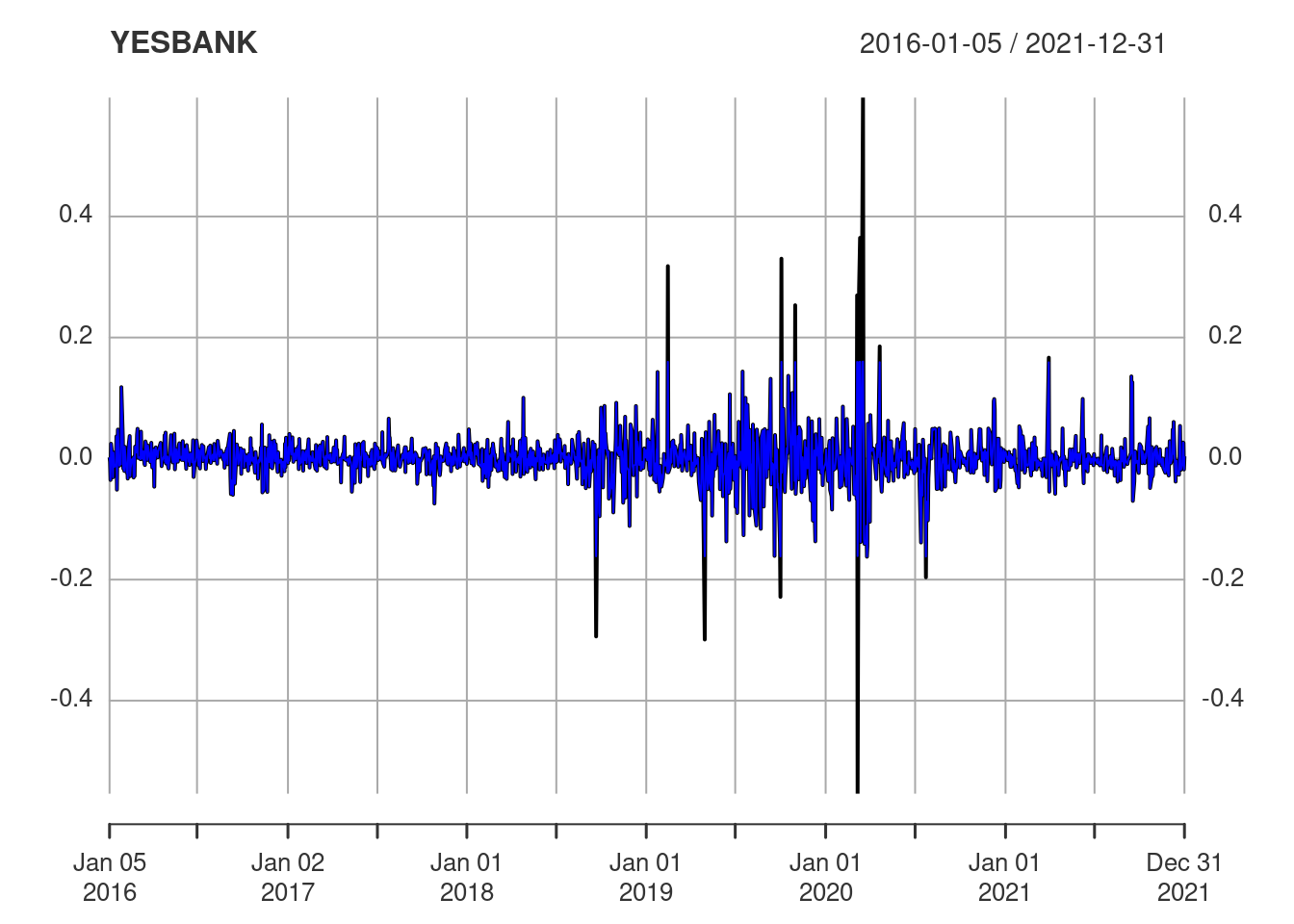
This can be appreciated by looking at the range (minimum and maximum values) of the raw and cleaned data.
range(YESBANK)[1] -0.5537634 0.5964912range(yesbank)[1] -0.1621622 0.1601474Importance of Volatility
Why is volatility important? It is an fundamental consideration in predicting future returns. Stocks with lower volatility are less likely to have substantial changes in return from day to day. However, stocks with higher volatility are literally more “volatile”: their returns can vary substantially from day to day.
As we have seen, volatility varies from stock to stock (some companies are more volatile than others) and from period to period (a company may have times of low and high volatility).
Volatility needs to be factored into future predictions. Of course, we also don’t know what future volatilities will be, so in addition to predicting future returns we will probably also want to predict future volatilities. We’ll see how this can be done in an upcoming post on GARCH models.