A GARCH (Generalised Autoregressive Conditional Heteroskedasticity) model is a statistical tool used to forecast volatility by analysing patterns in past price movements and volatility. The name itself feels intimidating (acronyms are a form of gatekeeping, right?), so let’s decompose it:
- Generalized — It’s an expanded version of earlier models that were more limited in scope.
- Autoregressive — It uses past values to predict future values.
- Conditional — Its assumes that future volatility depends on information from the past.
- Heteroskedasticity — It allows volatility to change over time (volatility is not constant). This means that it can handle periods of high (where prices are volatile) and low (where prices are stable) volatility.
GARCH models are typically used in risk management, portfolio optimisation, and financial decision-making, giving insights into how volatile an asset might be in the future.
Returns & Prediction Errors
A GARCH model effectively has two components:
- a model for the average return and
- a model for the return standard deviation (or volatility).
We’ll denote the observed returns by \(R_t\), where the subscript \(t\) indicates that this is the return for time period \(t\). The observed returns are described by an average return model, \(\bar{R}\). The difference between the observations and the model is the model residual (or prediction error), \(e_t\), which is also time dependent so it gets a \(t\) subscript too.
\[ R_t = \bar{R}_t + e_t. \]
A simple model might suppose that the returns are normally distributed and centred on the average return, \(\mu\). We can then write
\[ R_t = \mu + e_t \]
where the model residual is distributed as
\[ e_t \sim N(0, \sigma^2) \]
and \(\sigma\) is the return standard deviation.
This model assumes that the variability in the returns is constant. However, in practice this is a poor assumption. It makes more sense to assume that the prediction errors are normally distributed with a variance that changes with time, \(\sigma_t\):
\[ e_t \sim N(0, \sigma_t^2). \]
But now we need a model for \(\sigma_t\). The normal GARCH model sets
\[ \sigma_t^2 = \omega + \alpha e_{t-1}^2 + \beta \sigma_{t-1}^2. \]
The term with coefficient \(\alpha\) depends on the square of the lagged model residual. The term with coefficient \(\beta\) is the contribution of lagged volatility. This is the model for the conditional variance. It’s expected that the conditional variance will converge to a constant level, the unconditional variance, given by
\[ \frac{\omega}{1 - \alpha - \beta}. \]
The model has four parameters: \(\mu\), \(\omega\), \(\alpha\) and \(\beta\). The Maximum Likelihood method will be used to estimate the set of parameter values which are most likely to have generated the observed returns.
Data
We’ll use the same data as in the previous post in this series.
Packages
The {rugarch} and {tsgarch} packages will be used to build the models. The latter package is a partial rewrite of the former.
library(rugarch)
library(tsgarch)
Model: Constant Mean
First we need to set up the specifications of the model.
specification <- ugarchspec(
  distribution.model = "norm",
  mean.model = list(armaOrder = c(0, 0)),
  variance.model = list(model = "sGARCH")
)
That specifies a standard GARCH model with constant mean. Dissecting the parameters:
distribution.model— The distribution assumed for the returns, in this case a Normal Distribution. A Normal Distribution has both a mean and a variance. These are determined via themean.modelandvariance.modelparameters.mean.model— The model used to describe the mean. In this case we have specified an ARMA model with neither an autoregressive (AR) or moving average (MA) component. Since there is neither an autoregressive or moving average component, this model assumes that the mean is constant with time, and doesn’t depend on previous returns or a moving average of previous returns.variance.model— The model used to describe the variance. The “standard” GARCH model ("sGARCH") has been chosen. This model predicts volatility based on past volatility and past returns. This part of the model is what results in volatility clustering: if returns were volatile yesterday then they are likely to also be volatile today.
Next fit the model to the returns for Tata Steel, providing the model specification.
fit <- ugarchfit(data = TATASTEEL, spec = specification)The fit object has a number of utility methods which can be used to interrogate the model.
Coefficients
The model is fully specified by its coefficients. As mentioned above, there are four model parameters.
coef(fit) mu omega alpha1 beta1
1.484726e-03 1.242721e-05 4.152822e-02 9.373509e-01 The value of mu is the average return, while omega, alpha1 and beta1 correspond to \(\omega\), \(\alpha\) and \(\beta\) in the model above.
Fitted Mean
The model assumed that the average return is constant and this can be seen in the fitted value for \(\mu\).
fitted(fit)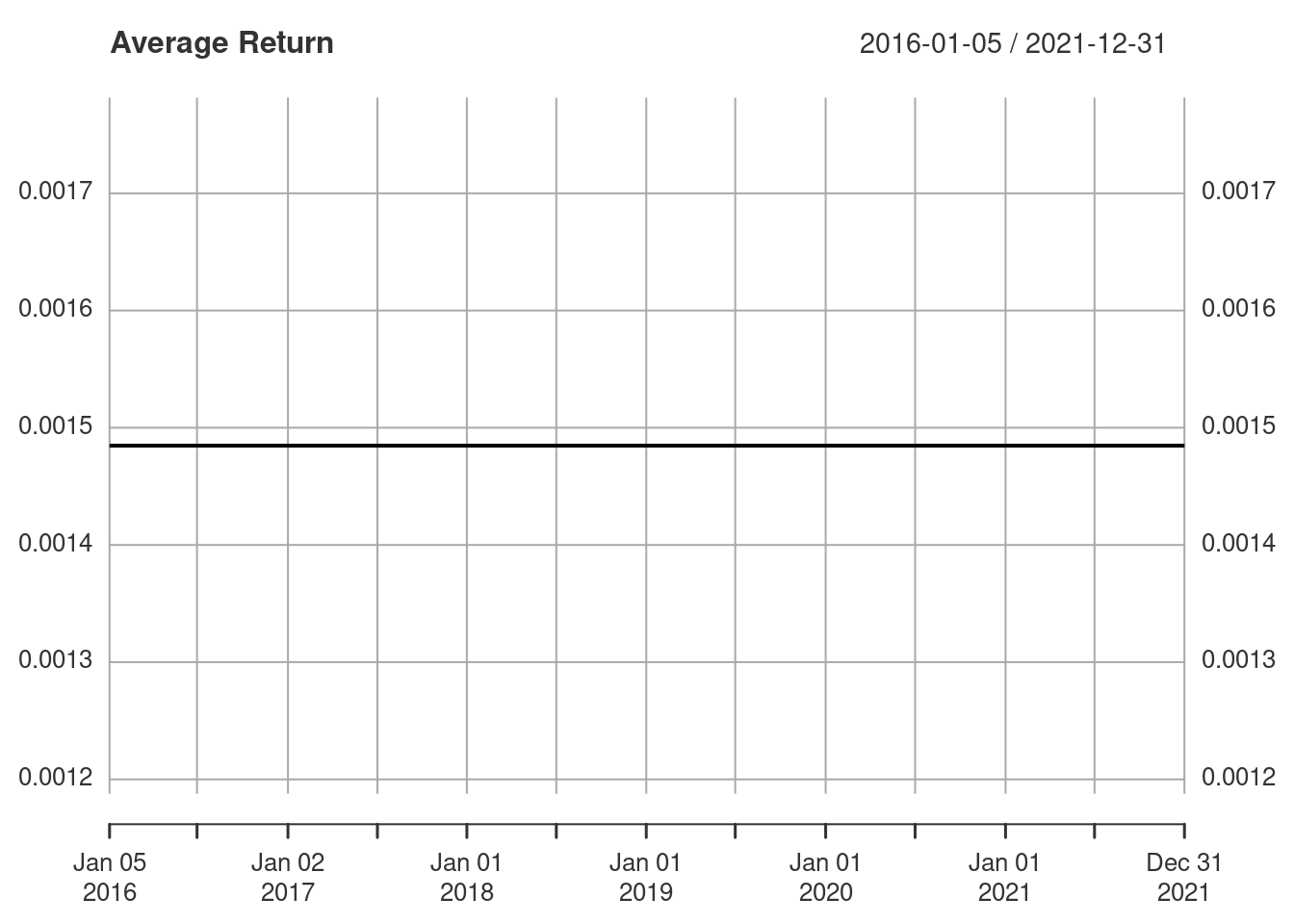
Fitted Volatility
Although the average return is assumed to be constant, the volatility changes with time.
sigma(fit)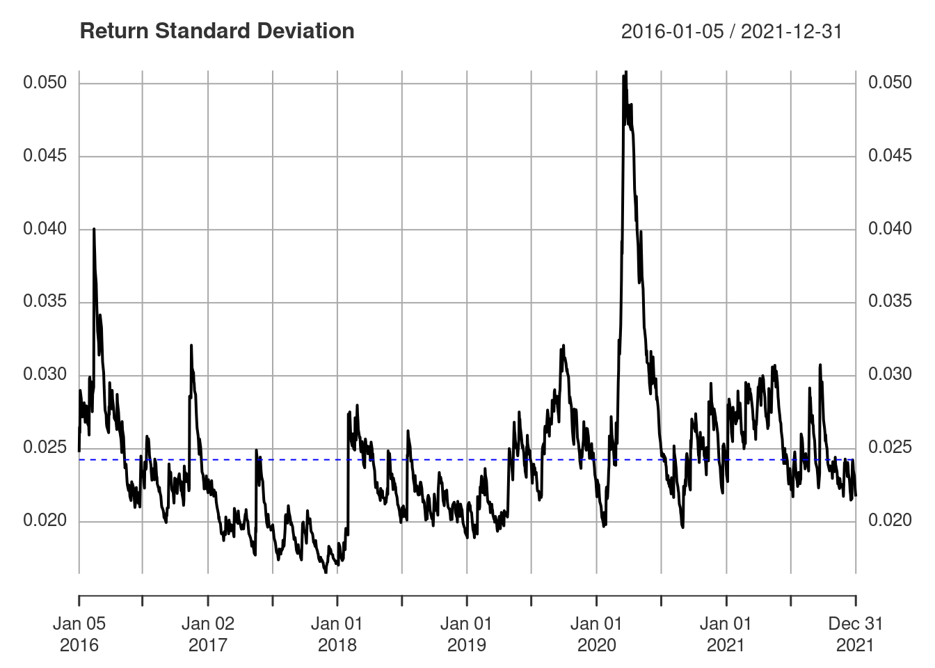
This can be compared with the volatility moving averages from the previous post, but in this case we have been somewhat more sophisticated in actually fitting a model to the volatility. The period of higher volatility in the first half of 2020 corresponds to the large fluctuations that are visible in the returns in the same period. Higher volatility ⇆ more variable returns.
Unconditional Volatility
The conditional volatility is mean reverting and returns to the unconditional volatility over the long term.
sqrt(uncvariance(fit))[1] 0.02425664The unconditional variance is plotted as a dashed blue line above.
Volatility Forecast
One of the primary applications of a model is to make predictions. Using ugarchforecast() we can predict future returns and volatility.
forecast <- ugarchforecast(fit, n.ahead = 10)
*------------------------------------*
*       GARCH Model Forecast         *
*------------------------------------*
Model: sGARCH
Horizon: 10
Roll Steps: 0
Out of Sample: 0

0-roll forecast [T0=2021-12-31]:
       Series   Sigma
T+1  0.001485 0.02140
T+2  0.001485 0.02147
T+3  0.001485 0.02153
T+4  0.001485 0.02159
T+5  0.001485 0.02165
T+6  0.001485 0.02171
T+7  0.001485 0.02177
T+8  0.001485 0.02182
T+9  0.001485 0.02188
T+10 0.001485 0.02193
The forecast object also has a suite of methods. For example, you can extract just the volatilities.
sigma(forecast) 2021-12-31
T+1 0.02140490
T+2 0.02146905
T+3 0.02153165
T+4 0.02159276
T+5 0.02165241
T+6 0.02171065
T+7 0.02176750
T+8 0.02182301
T+9 0.02187721
T+10 0.02193013Another Approach
Let’s perform a similar analysis using the {tsgarch} package. Again we start with a model specification.
specification <- garch_modelspec(
  TATASTEEL,
  model = "garch",
  constant = TRUE
)
That specifies a GARCH model with constant mean. Unlike with {rugarch} the returns data are baked into the specification. Now fit the model.
fit <- estimate(specification)And take a look at the model summary, which shows the estimates of the model parameters along with an indication of their statistical significance.
summary(fit)GARCH Model Summary
Coefficients:
Estimate Std. Error t value Pr(>|t|)
mu 1.485e-03 5.956e-04 2.494 0.01264 *
omega 1.250e-05 4.768e-06 2.622 0.00873 **
alpha1 4.163e-02 8.779e-03 4.742 2.11e-06 ***
beta1 9.371e-01 1.388e-02 67.512 < 2e-16 ***
persistence 9.788e-01 8.471e-03 115.542 < 2e-16 ***
---
Signif. codes: 0 '***' 0.001 '**' 0.01 '*' 0.05 '.' 0.1 ' ' 1
N: 1484
V(initial): 0.0006138, V(unconditional): 0.0005893
Persistence: 0.9788
LogLik: 3439.6, AIC: -6869.21, BIC: -6842.7Plotting the model gives a lot more information than what was available from the {rugarch} model.
plot(fit)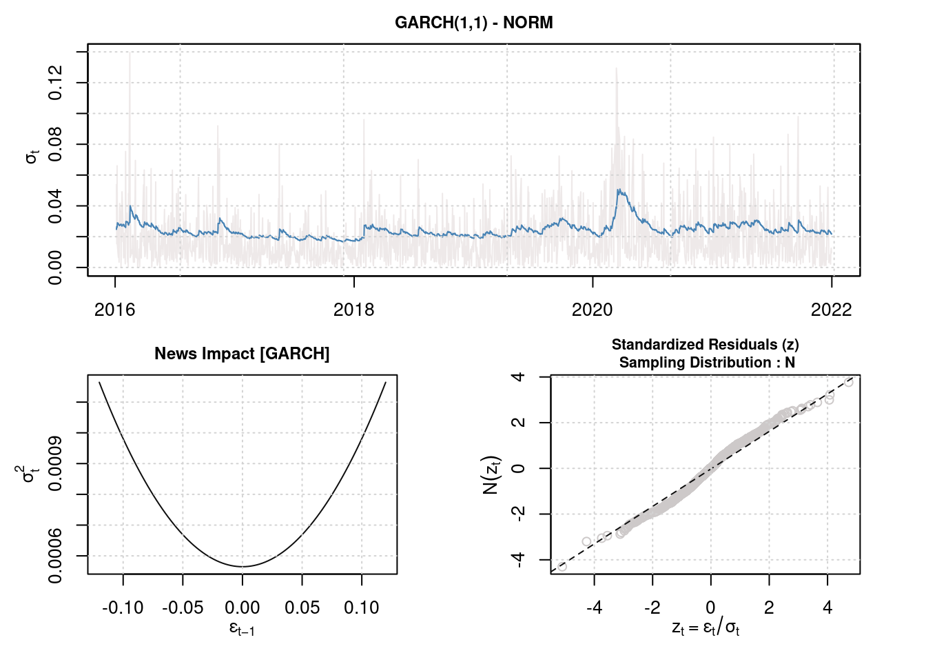
Conclusion
We have built a couple of GARCH models. We’ll dig into them further in upcoming posts.