In the previous post we assumed that returns had a normal distribution. This assumption implied that the distribution was symmetric and a positive return was as likely as the corresponding negative return. In reality this assumption is just not true and returns are asymmetrically distributed. It’s often said that
Markets take the stairs up, but the elevator down.
The implication is that markets usually increase in value gradually, like someone climbing up stairs step by step. But when they fall, they tend to do so very quickly, as if taking an elevator down. Positive returns tend to be smaller than negative returns.
Distribution Symmetry
Let’s take a look at the distribution of returns for ACC.
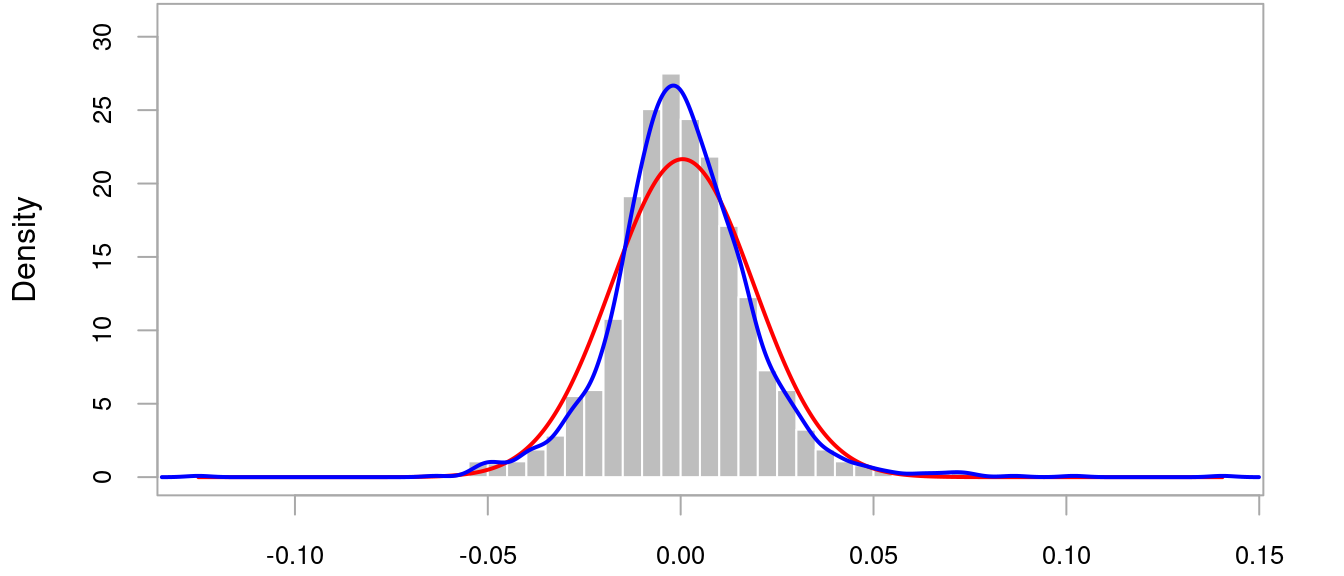
The gray bars are a histogram of the returns. The blue curve is the empirical density, which should be compared with the red curve which is the corresponding Normal Distribution. It’s apparent that the empirical distribution is more peaked around zero and has “fat tails”. It’s also not symmetric around zero.
To cater for an asymmetric distribution of returns we can change the distribution.model parameter from "norm" (for a Normal Distribution) to "sstd" (for a Skewed Student-t Distribution). The skewed distribution has two extra parameters:
\(\nu\)(shape) — determines the “fatness” and\(\xi\)(skew) — determines the “skewness”.
The Normal Distribution is a special case of the Skewed Student-t Distribution with \(\xi = 1\) and \(\nu = \infty\).
Comparing Distributions
Let’s first model those data using a Normal Distribution for the residuals.
specification <- ugarchspec(
  distribution.model = "norm",
  mean.model = list(armaOrder = c(0, 0)),
  variance.model = list(model = "sGARCH")
)

fit <- ugarchfit(data = ACC, spec = specification)

coef(fit)
mu omega alpha1 beta1
7.196519e-04 1.741614e-05 6.181566e-02 8.862315e-01 What’s the model likelihood? 💡 This is a measure of how likely the data are given a specific set of parameters. Bigger is better.
likelihood(fit)[1] 3884.409Now compare a Skewed Student-t Distribution.
specification <- ugarchspec(
  distribution.model = "sstd",
  mean.model = list(armaOrder = c(0, 0)),
  variance.model = list(model = "sGARCH")
)

fit <- ugarchfit(data = ACC, spec = specification)

coef(fit)
mu omega alpha1 beta1 skew shape
5.677503e-04 1.503252e-05 5.680452e-02 8.973454e-01 1.079020e+00 5.756512e+00 The parameters for the original model, \(\mu\), \(\omega\), \(\alpha\) and \(\beta\), are still present. But now we also have \(\nu\) and \(\xi\). The skewness, \(\xi\), indicates that the distribution is slightly asymmetric, while the shape, \(\nu\), suggests that the distribution has fatter tails than a Normal Distribution.
Get the likelihood for comparison.
likelihood(fit)[1] 3944.611A higher likelihood indicates that this is probably a better description of the data.
Conclusion
Choosing an appropriate distribution for the model residuals can make a big difference to model quality. Since the distribution of returns is generally not symmetric about zero a Skewed Student-t Distribution is often more appropriate than a Normal Distribution.